Chapter 9 Training and Testing Sets for Iris Data
set.seed(1120)
train=sample(150,105)
iris[train,]    #Training data  (70% of the data)
iris[-train,]   #Test data      (30% of the data)

#More general code for training set
train=sample(nrow(iris),round(0.7*nrow(iris),0))
Use training data to construct a tree.
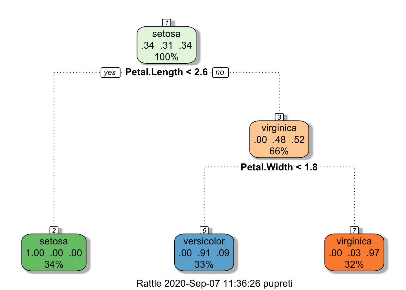
Using confmatrix function to calculate accuracy and error
#Confusion matrix, accuracy, and error rate for training data.
confmatrix(iris$Species[train],
           predict(iristree,newdata=iris[train,],type="class"))
## $matrix
## predy
## y setosa versicolor virginica
## setosa 36 0 0
## versicolor 0 32 1
## virginica 0 3 33
##
## $accuracy
## [1] 0.9619048
##
## $error
## [1] 0.03809524#Confusion matrix, accuracy, and error rate for test data.
confmatrix(iris$Species[-train],
predict(iristree,newdata=iris[-train,],type="class"))## $matrix
## predy
## y setosa versicolor virginica
## setosa 14 0 0
## versicolor 0 17 0
## virginica 0 2 12
##
## $accuracy
## [1] 0.9555556
##
## $error
## [1] 0.044444449.1 Example Data
Import traindata.csv and testdata.csv. Make sure class variable is a factor. And quick data exploration.
traindata = read.csv(url("http://faculty.tarleton.edu/crawford/documents/Math5364/traindata.csv"))
testdata = read.csv(url("http://faculty.tarleton.edu/crawford/documents/Math5364/testdata.csv"))
traindata$class=as.factor(traindata$class)
testdata$class=as.factor(testdata$class)

#Quick Data Exploration
dim(traindata)
## [1] 900 3## x y class
## 1 4.76295819 9.583156 0
## 2 9.77532792 8.282632 0
## 3 0.05409077 18.185264 0
## 4 16.48119755 16.129525 0
## 5 12.87665297 16.614146 1
## 6 8.61560780 3.930424 1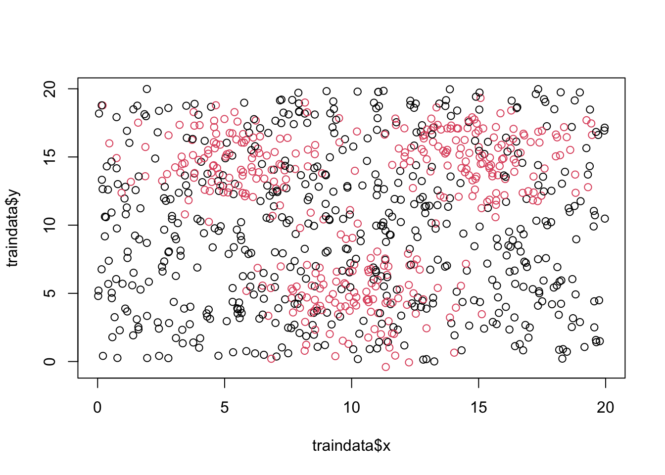
## [1] 2100 3## x y class
## 1 17.9655968 3.183029 0
## 2 6.6738789 6.675273 1
## 3 10.2086342 8.073150 0
## 4 0.7836262 2.630917 0
## 5 13.1109049 7.214607 0
## 6 4.2286522 13.943382 1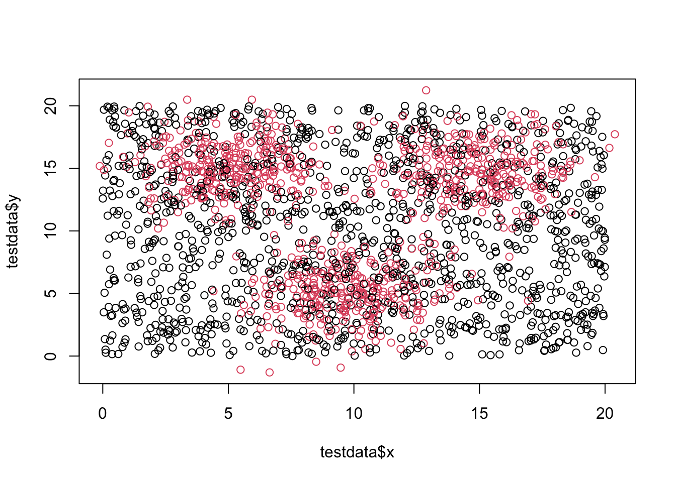
Building Tree 1 from the Slides
## $matrix
##    predy
## y     0   1
##   0 414 125
##   1  67 294
##
## $accuracy
## [1] 0.7866667
##
## $error
## [1] 0.2133333## $matrix
## predy
## y 0 1
## 0 873 388
## 1 224 615
##
## $accuracy
## [1] 0.7085714
##
## $error
## [1] 0.2914286Number of Nodes for Tree 1
#extree1$frame #Frame of information about the nodes
dim(extree1$frame) #First entry tells us how many nodes there are## [1] 27 9Class Breakdown for Training and Testing Data
##
## 0 1
## 0.5988889 0.4011111##
## 0 1
## 0.6004762 0.3995238## [1] 900## [1] 21009.2 Statistical tests to test the model
9.2.1 Confidence Intervals for Classification Accuracy
Exact binomial test. Example test data had 2100 records, and 1488 were classified correctly. The confidence interval based on the binomial distribution
## $matrix
##    predy
## y     0   1
##   0 873 388
##   1 224 615
##
## $accuracy
## [1] 0.7085714
##
## $error
## [1] 0.2914286##
## Exact binomial test
##
## data: 1488 and 2100
## number of successes = 1488, number of trials = 2100, p-value < 2.2e-16
## alternative hypothesis: true probability of success is not equal to 0.5
## 95 percent confidence interval:
## 0.6886162 0.7279429
## sample estimates:
## probability of success
## 0.7085714Building tree 2
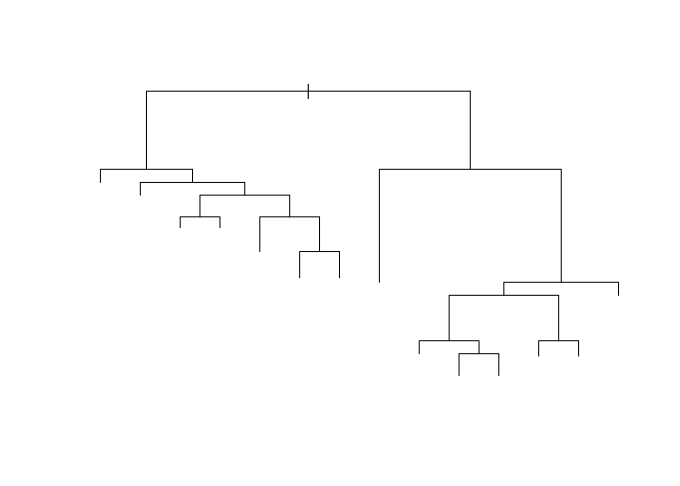
extree2=rpart(class~.,data=traindata,
              control=rpart.control(minsplit=1,cp=0))
fancyRpartPlot(extree2)
## Warning: labs do not fit even at cex 0.15, there may be some overplotting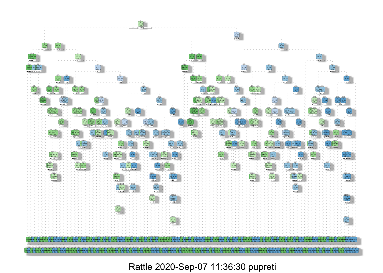
## $matrix
##    predy
## y     0   1
##   0 539   0
##   1   0 361
##
## $accuracy
## [1] 1
##
## $error
## [1] 0## $matrix
## predy
## y 0 1
## 0 883 378
## 1 338 501
##
## $accuracy
## [1] 0.6590476
##
## $error
## [1] 0.3409524Building accuracy vectors
## accvector1
## FALSE  TRUE
## 612 1488## accvector1
## FALSE TRUE
## 0.2914286 0.7085714## accvector2
## FALSE TRUE
## 716 1384## accvector2
## FALSE TRUE
## 0.3409524 0.6590476McNemar Table
##           accvector2
## accvector1 FALSE TRUE
##      FALSE   438  174
##      TRUE    278 1210
Chi-square statistic and p-value
## [1] 23.47124## [1] 1.267952e-06Built-in Function
##
## 	McNemar's Chi-squared test with continuity correction
##
## data:  mcnemartable
## McNemar's chi-squared = 23.471, df = 1, p-value = 1.268e-06
Exact McNemar Test
##
## 	Exact McNemar test (with central confidence intervals)
##
## data:  mcnemartable
## b = 174, c = 278, p-value = 1.144e-06
## alternative hypothesis: true odds ratio is not equal to 1
## 95 percent confidence interval:
##  0.5148605 0.7591830
## sample estimates:
## odds ratio
##  0.6258993
9.3 10-fold Cross-validation
Combine traindata and testdata.
library(cvTools)
Exdata=rbind(traindata,testdata)
folds=cvFolds(nrow(Exdata),K=10,type='random')


#createfolds function
createfolds=function(n,K){
  reps=ceiling(n/K)
  folds=sample(rep(1:K,reps))
  return(folds[1:n])
}

#Folds for Exdata
set.seed(5364)
folds=createfolds(nrow(Exdata),10)
Accuracy for first fold
## [1] 300 3## [1] 2700 3## x y
## 29827.02 31738.17## x y
## 29827.02 31738.17temptree=rpart(class~.,data=temptrain)
tempacc=confmatrix(temptest$class,
predict(temptree,newdata=temptest,type="class"))$accuracy
tempacc## [1] 0.6966667Accuracy for all folds using a loop.
accvector=1:10

for(k in 1:10){
  temptest=Exdata[folds==k,]
  temptrain=Exdata[folds!=k,]

  temptree=rpart(class~.,data=temptrain)
  accvector[k]=confmatrix(temptest$class,
                     predict(temptree,newdata=temptest,type="class"))$accuracy
}

mean(accvector)
## [1] 0.7146667Delete-d Hints. Let d=20
index=sample(nrow(Exdata))
index[1:20]
index[21:nrow(Exdata)]
Bootstrap Hints
index=sample(nrow(Exdata),replace=TRUE)