Chapter 4 Linear Regression

Concepts:

• Regression Line
• Correlation
• Mean Squared Errors and Root Mean Squared Errors
• Estimate \(\hat{\sigma}\)
• Ordinary Least Squares (OLS) Estimator \(\hat{\beta}\) BLUE
• Covariance matrix \(\widehat{cov}(\hat{\beta})\)
• Standard Error
• Model output (t-values, p-values, F-statistics, p-value of F-statistic)
• OLS Assumptions

---

4.1 Simple Linear Regression

Lets look at the Old faithful eruptions data again. In the dataset have eruption duration (mins) and waiting time between each eruption. We can look at the scatterplot and the line that best describes the pattern

eruptions	waiting
3.600	79
1.800	54
3.333	74
2.283	62
4.533	85
2.883	55

ggplot(faithful, aes(x= waiting, y = eruptions)) + 
  geom_point() +
  geom_smooth(method = 'lm', formula = y~x)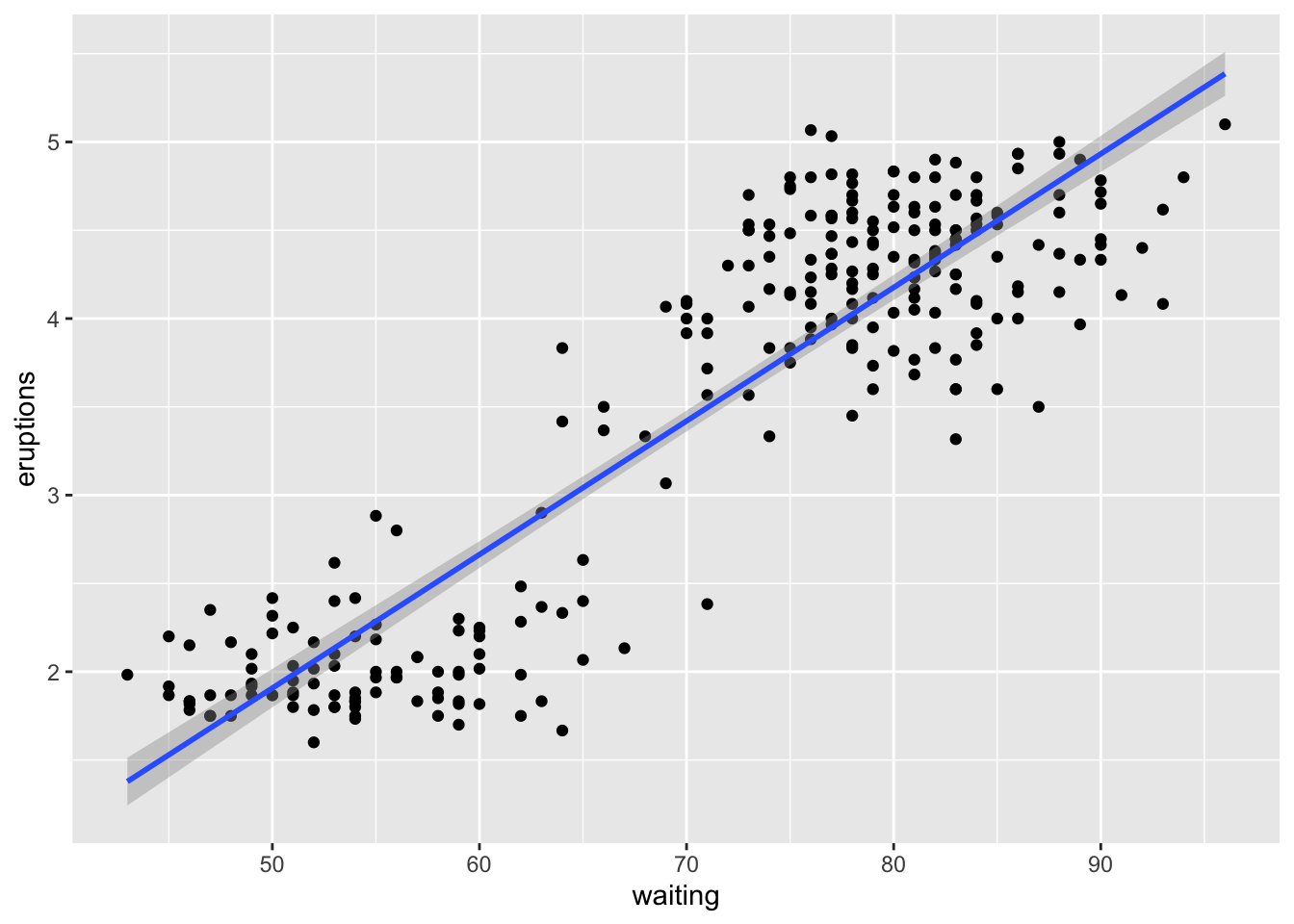

Here we can see that the length of the eruptions are “positively correlated” with the waiting time i.e. longer the waiting time, longer the eruptions. We can also see that the points are clustered around two areas. The line that best fits the data is known as regression line.

We can do some basic calculations to build this linear model using r.

Mean Eruption times = 3.4877831
Variance Eruption times = 1.3027283
Standard Deviation of Eruption times = 1.1413713
Mean wait times = 70.8970588
Variance wait times = 184.8233124
Standard Deviation of wait times = 13.5949738
Correlation coefficient = 0.8974994
Slope of regression line =
Mean Square Errors

Running inbuilt function to run linear regression

simple_linear = lm(formula = eruptions~waiting, data = faithful)
summary(simple_linear)

## 
## Call:
## lm(formula = eruptions ~ waiting, data = faithful)
## 
## Residuals:
##      Min       1Q   Median       3Q      Max 
## -1.29917 -0.37689  0.03508  0.34909  1.19329 
## 
## Coefficients:
##              Estimate Std. Error t value Pr(>|t|)    
## (Intercept) -1.874016   0.160143  -11.70   <2e-16 ***
## waiting      0.075628   0.002219   34.09   <2e-16 ***
## ---
## Signif. codes:  0 '***' 0.001 '**' 0.01 '*' 0.05 '.' 0.1 ' ' 1
## 
## Residual standard error: 0.4965 on 270 degrees of freedom
## Multiple R-squared:  0.8115,	Adjusted R-squared:  0.8108 
## F-statistic:  1162 on 1 and 270 DF,  p-value: < 2.2e-16

Explanation of the model here {residuals, coefficients, Standard-errors (including residuals), significance, F-statistic}

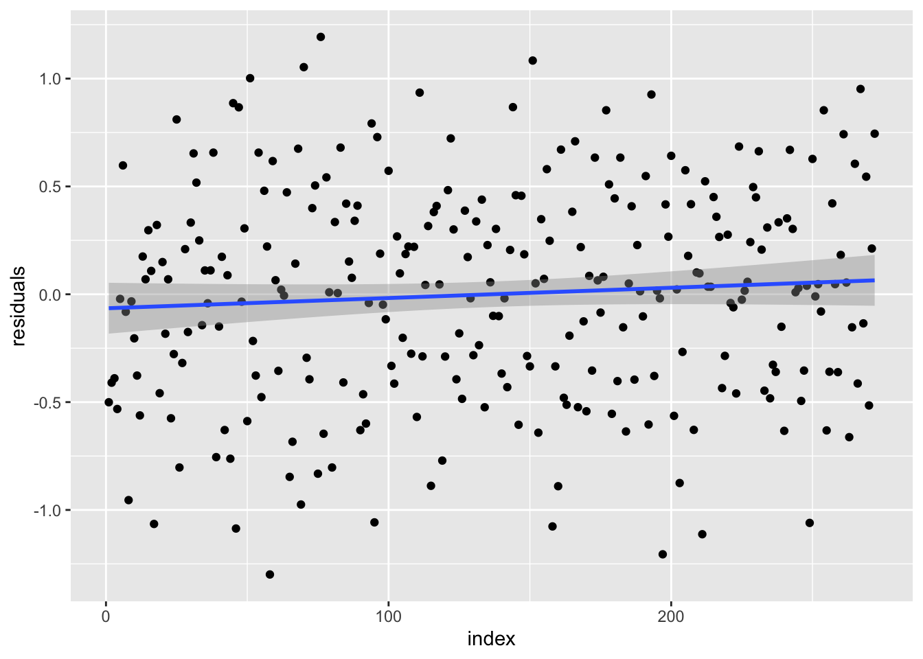
Residual plot

data.frame(index=index(simple_linear$residuals), residuals = simple_linear$residuals) %>% ggplot(., aes(x=index, y = residuals)) + geom_point() + geom_smooth(method = 'lm', formula = y~x)

---

4.2 Multiple Linear Regression

Extend simple linear regression to multiple linear regression.

Functional form \[y_i = \beta_1x_{i1} + ... \beta_px_{ip} + \epsilon_i \] We do not know true beta

\[Y = X\beta + \epsilon\] So we use \(\hat\beta\) to estimate \(\beta\) and OLS gives us the best result. Sum of squred of errors is minimized when \(\hat\beta = (X'X)^{-1}X'Y\)

Residuals \(e= Y - X\hat\beta\) and e is orthogonal to X

Ordinary Least Squares (involves some Matrix Algebra and mathematical proofs). Assumptions:
- Design matrix X has full rank. ie. there are more rows of data than the number of independent variables (features) in the dastaset - The unobservable random vector \(\epsilon\) is Independent and Identically distributed (IID) with mean 0 and variance of more than 0. - If design matrix X is random then \(\epsilon\) is independent of X.

Clarify the the difference between beta/betahat and e/epsilon

When the disturbance terms epsilon are normally distributed, the beta hat are the Maximum likely estimator for beta

Gradient Decent method Elaborate later

Define Loss Function Loss = residual . Calculate the Mean Squared of Errors

\[ E = \frac 1 n \sum_{i=0}^n(y_i - \bar y_i)^2 = \frac 1 n \sum_{i=0}^n(y_i - (mx_i +c))^2 \] Calculate the Gradient ie. partial derivative with respect to m and c to find the constants where the \(E\) is the smallest. Which are

\(D_m = \delta_m/\delta_y = \frac {-2} n \sum_{i=0}^n x_i(y_i - \bar y_i)\)

\(D_c = \delta_c/\delta_y = \frac {-2} n \sum_{i=0}^n (y_i - \bar y_i)\)

Update \(m\) and \(c\) using \(m = m - L \times D_m\) and \(c=c-L \times D_c\)

Repeat the \(m\) and \(c\) caluclation, plug the value into Loss function with value of x and y. The required \(m\) and \(c\) are when \(E = 0\).

Also need to avoid the local minima values so use multiple random starting point for values of \(m\) and \(c\) and do calculation multiple times (epochs)

Few things to test to ensure model fit

• plot residual vs x (should have no trend)
• Mean of residul should center around zero
• Assumption that residual are normally distributed

4.2.1 Consequences of Incorrect Functional Form

Creating data

set.seed(5366)
x=1:100
X=cbind(1,x,x^2)
beta=c(10,-1.15,0.0205)
y=X%*%beta+5*rnorm(100)
mydata=data.frame(y,x)

#Plot
plot(y~x,data=mydata)

#Fitting Quadratic Model
model2=lm(y~x+I(x^2),data=mydata)
summary(model2)

## 
## Call:
## lm(formula = y ~ x + I(x^2), data = mydata)
## 
## Residuals:
##     Min      1Q  Median      3Q     Max 
## -9.6521 -3.2214 -0.1858  2.9871 11.4882 
## 
## Coefficients:
##              Estimate Std. Error t value Pr(>|t|)    
## (Intercept) 11.453364   1.428003   8.021 2.43e-12 ***
## x           -1.208440   0.065264 -18.516  < 2e-16 ***
## I(x^2)       0.020854   0.000626  33.311  < 2e-16 ***
## ---
## Signif. codes:  0 '***' 0.001 '**' 0.01 '*' 0.05 '.' 0.1 ' ' 1
## 
## Residual standard error: 4.665 on 97 degrees of freedom
## Multiple R-squared:  0.9774,	Adjusted R-squared:  0.9769 
## F-statistic:  2098 on 2 and 97 DF,  p-value: < 2.2e-16

plot(y~x,data=mydata)

x.plot.vector=1:100
y.plot.vector=predict(model2,
                      newdata=data.frame(x=x.plot.vector))
lines(x.plot.vector,
      y.plot.vector,
      col="red")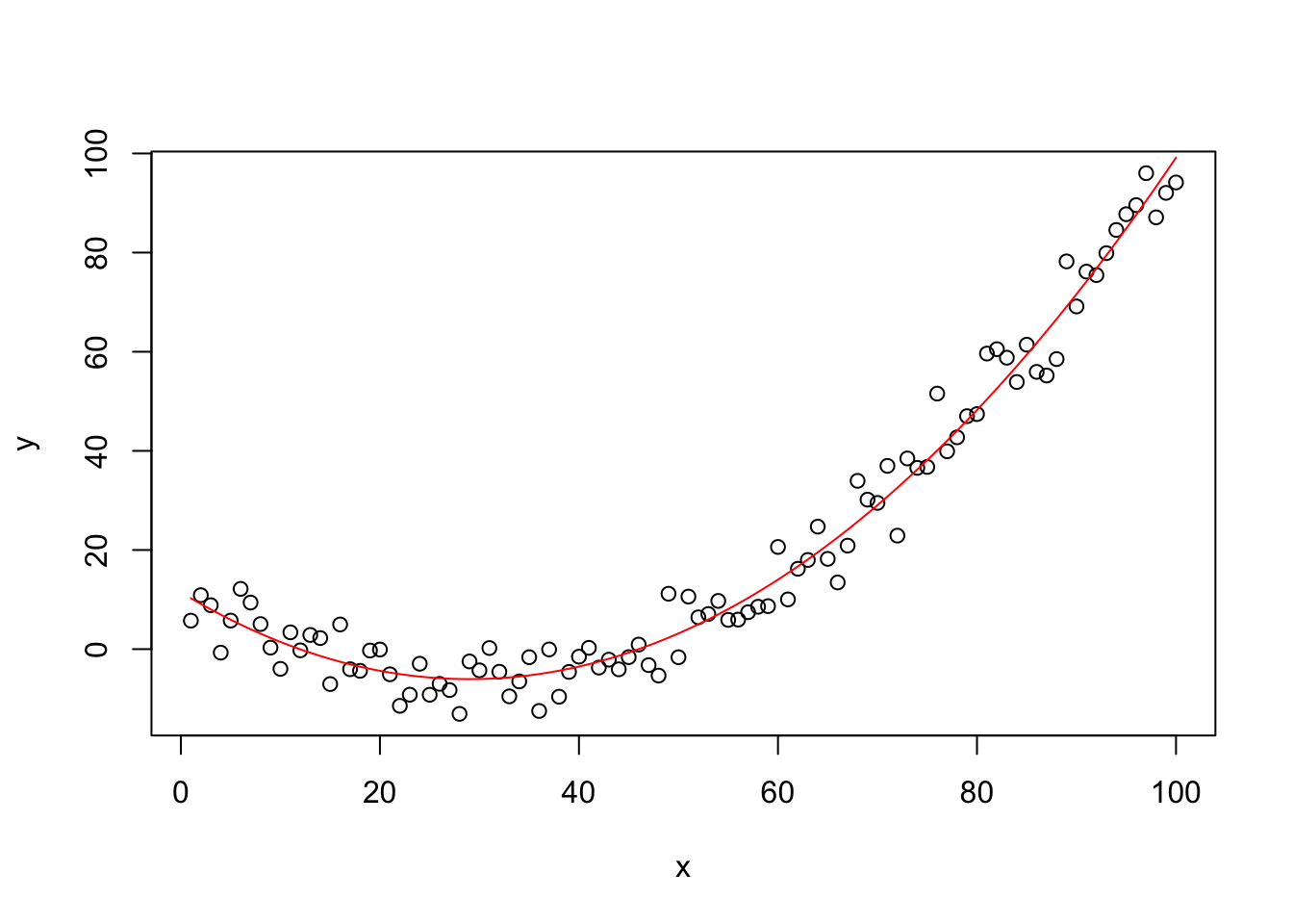

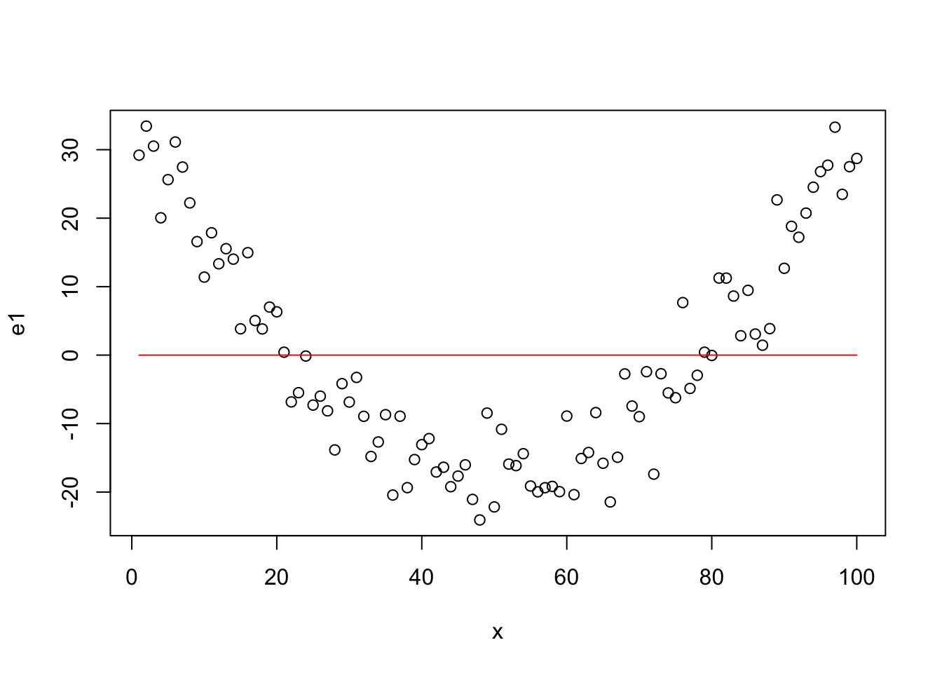
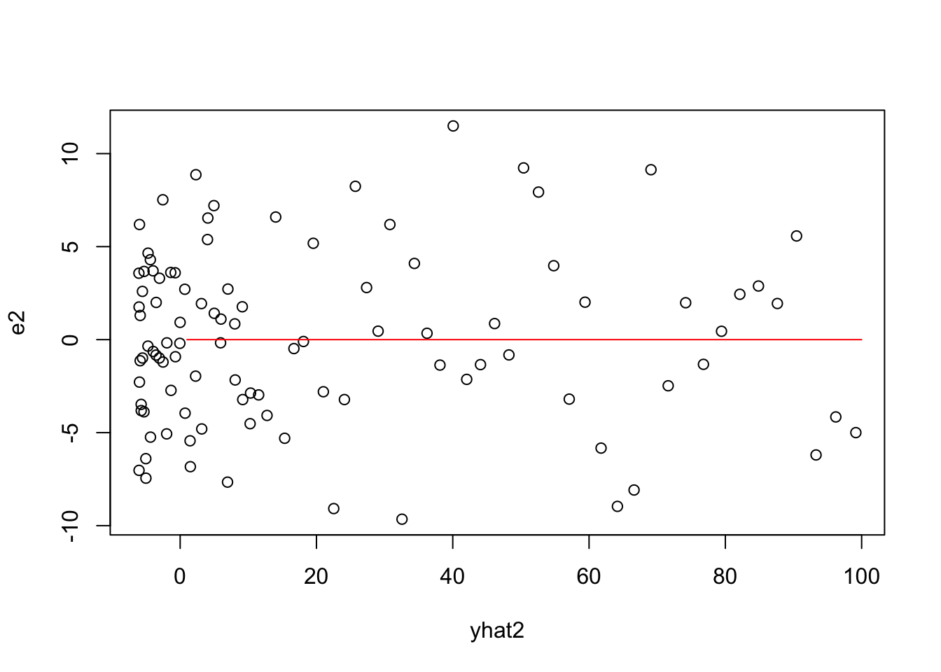
Residuals for Quadratic Model

betahat2=coef(model2)
X2=model.matrix(model2)

e2=y-X2%*%betahat2
#e2
e2=residuals(model2)
#e2

plot(x,e2)
lines(x,rep(0,length(x)),col="red")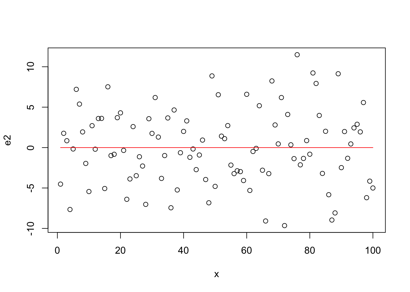

Fitting a linear model

plot(y~x,data=mydata)

model1=lm(y~x,data=mydata)
summary(model1)

## 
## Call:
## lm(formula = y ~ x, data = mydata)
## 
## Residuals:
##     Min      1Q  Median      3Q     Max 
## -24.077 -14.502  -3.712  12.844  33.444 
## 
## Coefficients:
##              Estimate Std. Error t value Pr(>|t|)    
## (Intercept) -24.35330    3.29860  -7.383 5.13e-11 ***
## x             0.89783    0.05671  15.833  < 2e-16 ***
## ---
## Signif. codes:  0 '***' 0.001 '**' 0.01 '*' 0.05 '.' 0.1 ' ' 1
## 
## Residual standard error: 16.37 on 98 degrees of freedom
## Multiple R-squared:  0.7189,	Adjusted R-squared:  0.7161 
## F-statistic: 250.7 on 1 and 98 DF,  p-value: < 2.2e-16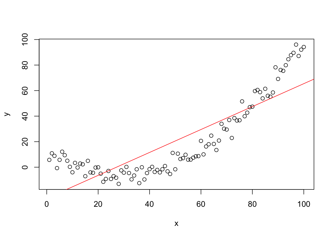

abline(model1,col="red")

#Residuals for Linear Model
e1=residuals(model1)

plot(x,e1)
lines(x,rep(0,length(x)),col="red")

f-test Function

ftest=function(model0,model){
  d0=length(coef(model0))
  d=length(coef(model))
  n=length(residuals(model))
  F=((deviance(model0)-deviance(model))/(d-d0))/
    ((deviance(model))/(n-d))
  return(pf(F,d-d0,n-d,lower.tail=FALSE))
}

ftest(model1,model2)

## [1] 6.724646e-55

summary(model2)

## 
## Call:
## lm(formula = y ~ x + I(x^2), data = mydata)
## 
## Residuals:
##     Min      1Q  Median      3Q     Max 
## -9.6521 -3.2214 -0.1858  2.9871 11.4882 
## 
## Coefficients:
##              Estimate Std. Error t value Pr(>|t|)    
## (Intercept) 11.453364   1.428003   8.021 2.43e-12 ***
## x           -1.208440   0.065264 -18.516  < 2e-16 ***
## I(x^2)       0.020854   0.000626  33.311  < 2e-16 ***
## ---
## Signif. codes:  0 '***' 0.001 '**' 0.01 '*' 0.05 '.' 0.1 ' ' 1
## 
## Residual standard error: 4.665 on 97 degrees of freedom
## Multiple R-squared:  0.9774,	Adjusted R-squared:  0.9769 
## F-statistic:  2098 on 2 and 97 DF,  p-value: < 2.2e-16

Plots involving Yhat for Quadratic Model

X2 = model.matrix(model2)
betahat2=coef(model2)
yhat2=X2%*%betahat2

plot(yhat2,y)
lines(1:100,1:100,col="red")

plot(yhat2,e2)
lines(1:100,rep(0,100),col="red")

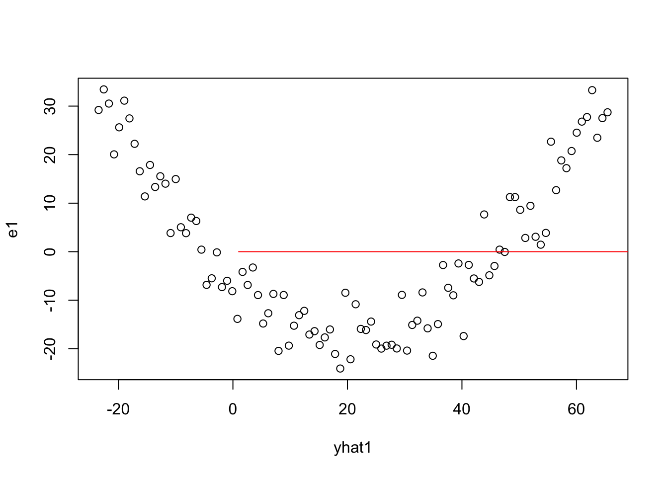
Plots involving Yhat for Linear Model

X1 = model.matrix(model1)
betahat1=coef(model1)
yhat1=X1%*%betahat1

plot(yhat1,y)
lines(1:100,1:100,col="red")

plot(yhat1,e1)
lines(1:100,rep(0,100),col="red")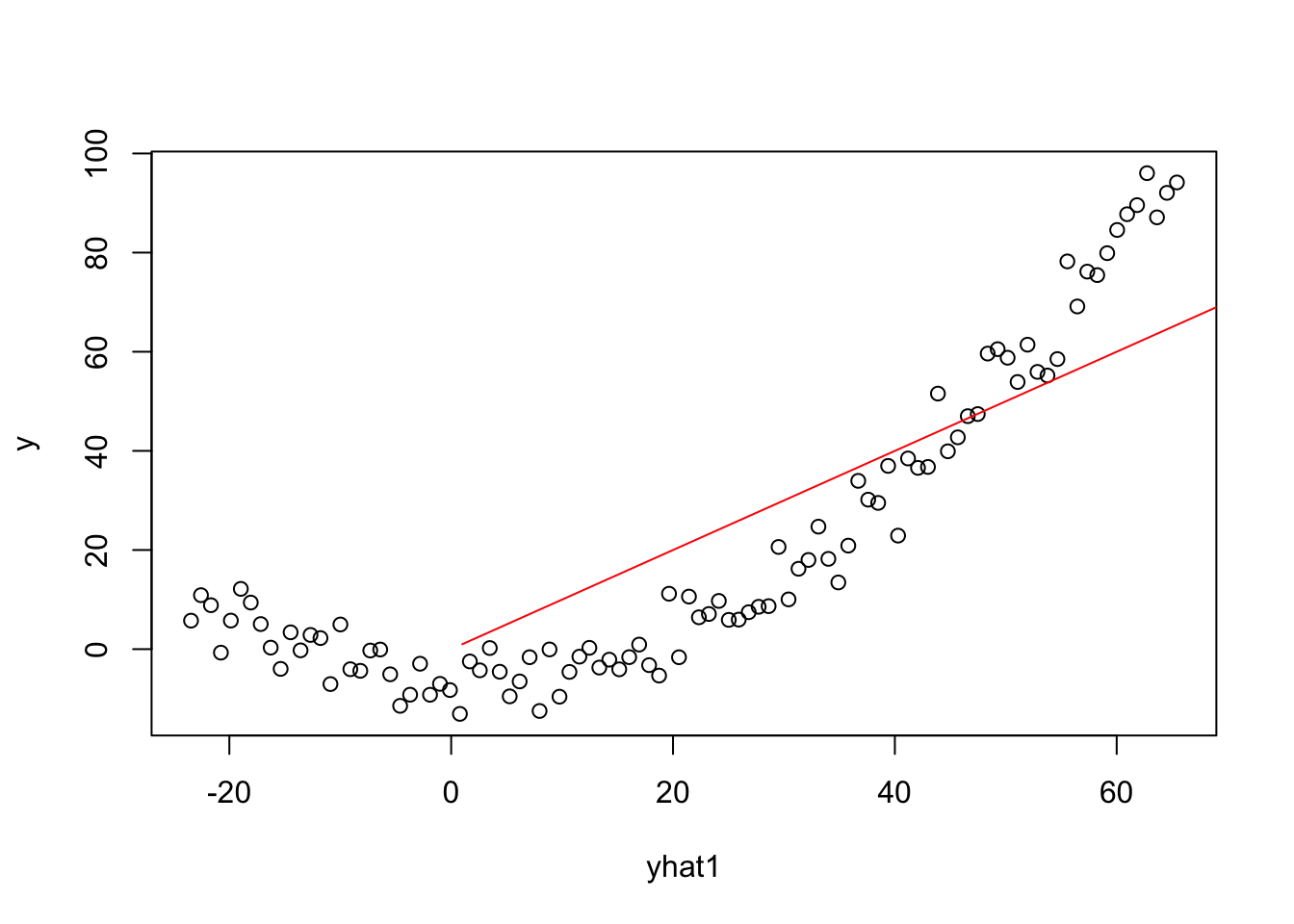

4.2.2 Design Matrix Assumptions

Rank of Design Matrix for Model2

library(Matrix)

head(X2)

##   (Intercept) x I(x^2)
## 1           1 1      1
## 2           1 2      4
## 3           1 3      9
## 4           1 4     16
## 5           1 5     25
## 6           1 6     36

dim(X2)

## [1] 100   3

rankMatrix(X2)

## [1] 3
## attr(,"method")
## [1] "tolNorm2"
## attr(,"useGrad")
## [1] FALSE
## attr(,"tol")
## [1] 2.220446e-14

#Model without Full Rank
z=x
model3=lm(y~x+I(x^2)+z)

X3=model.matrix(model3)

head(X3)

##   (Intercept) x I(x^2) z
## 1           1 1      1 1
## 2           1 2      4 2
## 3           1 3      9 3
## 4           1 4     16 4
## 5           1 5     25 5
## 6           1 6     36 6

dim(X3)

## [1] 100   4

rankMatrix(X3)

## [1] 3
## attr(,"method")
## [1] "tolNorm2"
## attr(,"useGrad")
## [1] FALSE
## attr(,"tol")
## [1] 2.220446e-14

summary(model3)

## 
## Call:
## lm(formula = y ~ x + I(x^2) + z)
## 
## Residuals:
##     Min      1Q  Median      3Q     Max 
## -9.6521 -3.2214 -0.1858  2.9871 11.4882 
## 
## Coefficients: (1 not defined because of singularities)
##              Estimate Std. Error t value Pr(>|t|)    
## (Intercept) 11.453364   1.428003   8.021 2.43e-12 ***
## x           -1.208440   0.065264 -18.516  < 2e-16 ***
## I(x^2)       0.020854   0.000626  33.311  < 2e-16 ***
## z                  NA         NA      NA       NA    
## ---
## Signif. codes:  0 '***' 0.001 '**' 0.01 '*' 0.05 '.' 0.1 ' ' 1
## 
## Residual standard error: 4.665 on 97 degrees of freedom
## Multiple R-squared:  0.9774,	Adjusted R-squared:  0.9769 
## F-statistic:  2098 on 2 and 97 DF,  p-value: < 2.2e-16

#Multicollinearity
w=x+rnorm(100)
plot(x,w)

cor(x,w)

## [1] 0.9993595

model4=lm(y~x+I(x^2)+w)
summary(model4)

## 
## Call:
## lm(formula = y ~ x + I(x^2) + w)
## 
## Residuals:
##     Min      1Q  Median      3Q     Max 
## -9.5002 -3.2165 -0.2137  2.9738 10.7425 
## 
## Coefficients:
##               Estimate Std. Error t value Pr(>|t|)    
## (Intercept) 11.5987222  1.4380446   8.066 2.06e-12 ***
## x           -1.6267839  0.4624638  -3.518 0.000667 ***
## I(x^2)       0.0208978  0.0006284  33.256  < 2e-16 ***
## w            0.4130417  0.4520250   0.914 0.363133    
## ---
## Signif. codes:  0 '***' 0.001 '**' 0.01 '*' 0.05 '.' 0.1 ' ' 1
## 
## Residual standard error: 4.669 on 96 degrees of freedom
## Multiple R-squared:  0.9776,	Adjusted R-squared:  0.9769 
## F-statistic:  1397 on 3 and 96 DF,  p-value: < 2.2e-16

4.2.3 NORMALITY OF ERROR TERMS

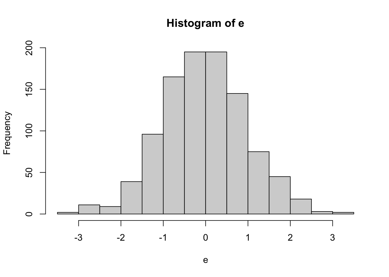
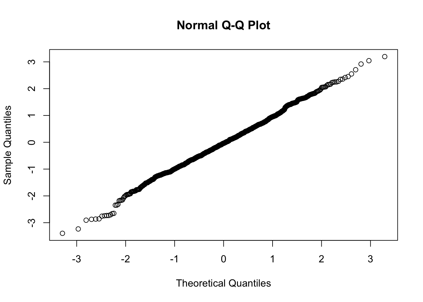
Normal Data

set.seed(1234)
e=rnorm(1000)
hist(e)

qqnorm(e)

shapiro.test(e)

## 
## 	Shapiro-Wilk normality test
## 
## data:  e
## W = 0.99737, p-value = 0.1053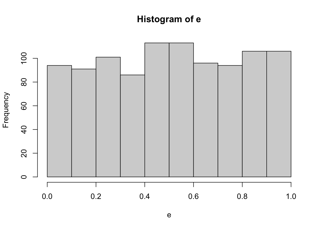

#Uniform Data
e=runif(1000)
hist(e)

qqnorm(e)

shapiro.test(e)

## 
## 	Shapiro-Wilk normality test
## 
## data:  e
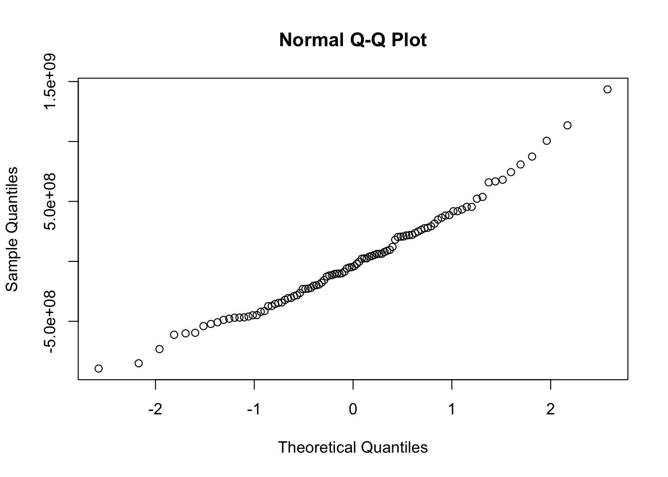
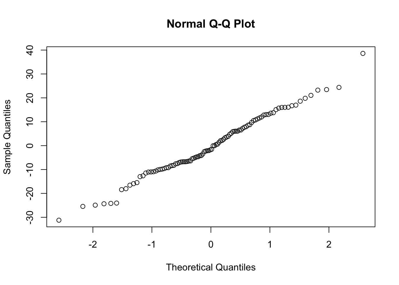
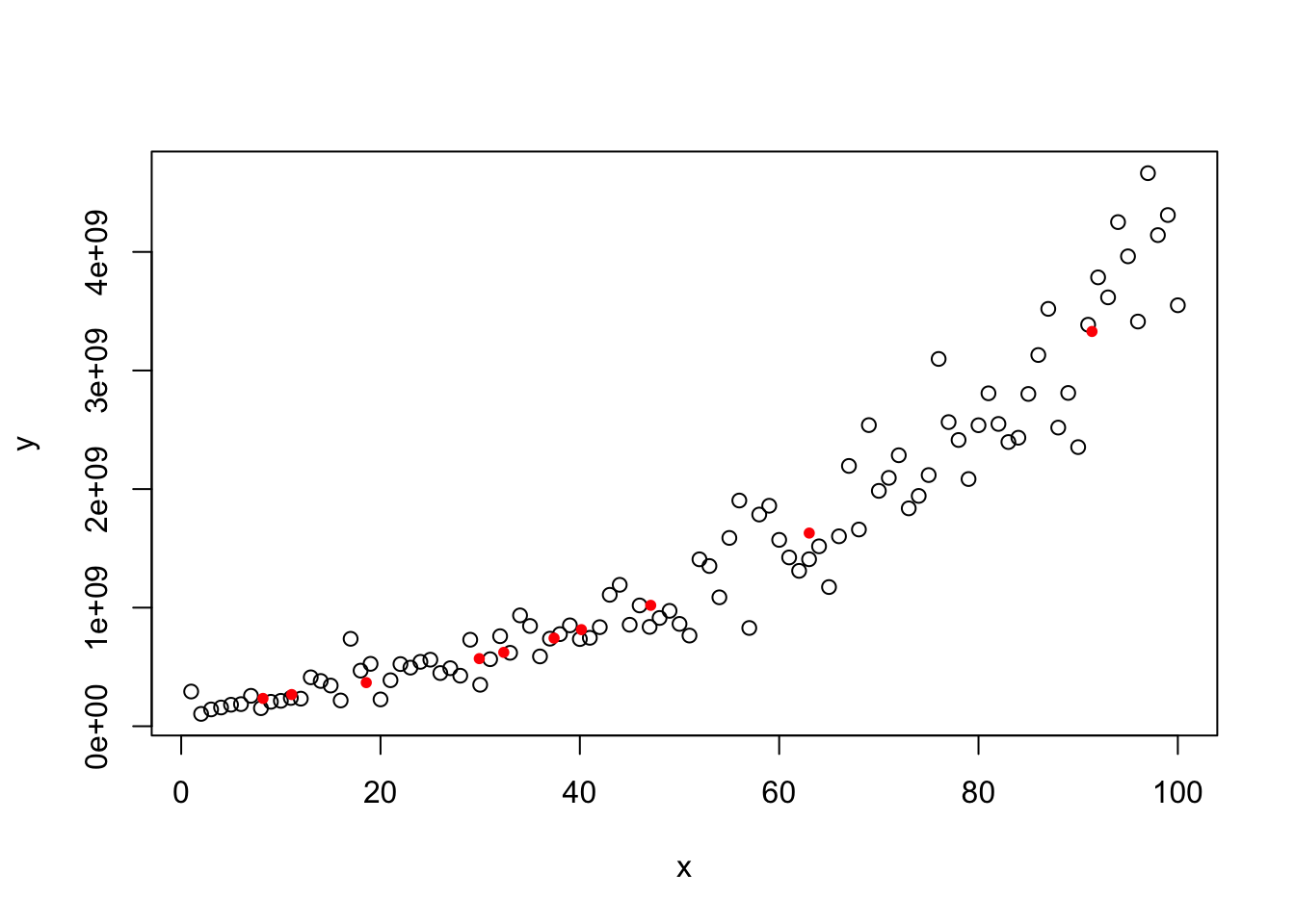
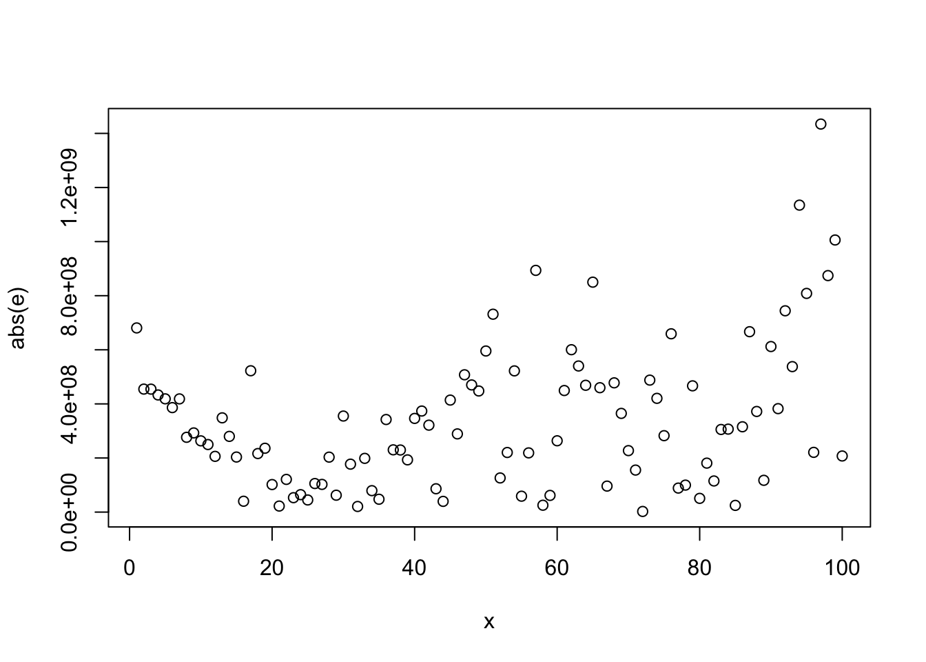
## W = 0.95765, p-value < 2.2e-16

#Model with Nonnormal Errors
x=1:100
y=(200+3*x+20*rnorm(100))^3.56
plot(x,y)

model=lm(y~x)
abline(model,col="red")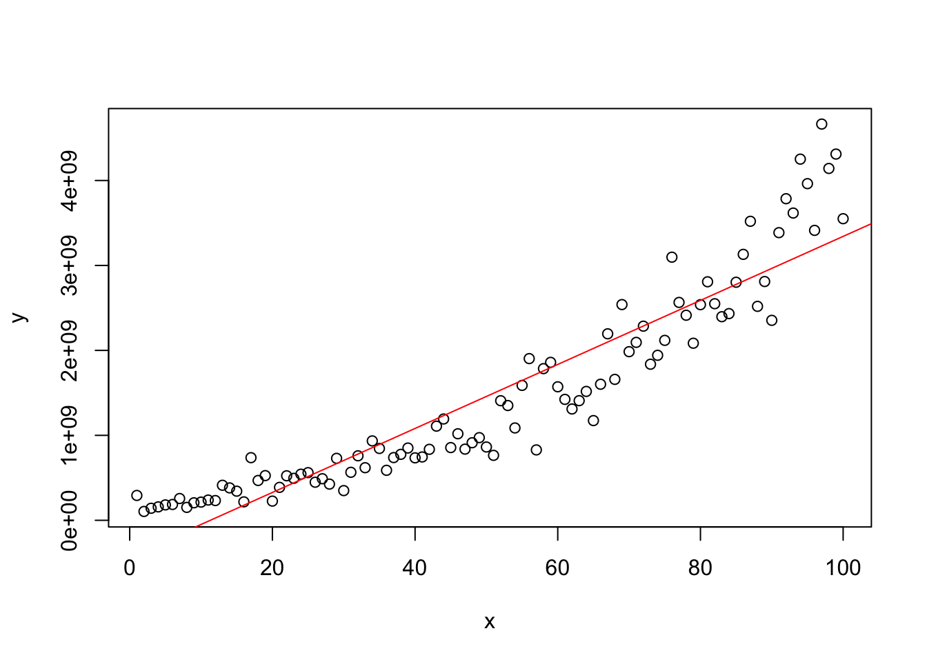

e=residuals(model)

qqnorm(e)

shapiro.test(e)

## 
## 	Shapiro-Wilk normality test
## 
## data:  e
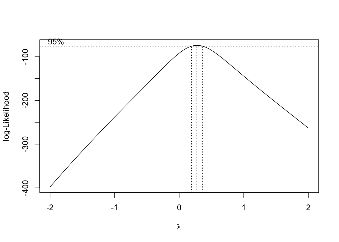
## W = 0.9762, p-value = 0.06698

Achieving Normality with Box-Cox Transformations

library(MASS)

boxcox.results=boxcox(model)

cbind(boxcox.results$x,boxcox.results$y)

##               [,1]       [,2]
##   [1,] -2.00000000 -397.92136
##   [2,] -1.95959596 -391.07290
##   [3,] -1.91919192 -384.25863
##   [4,] -1.87878788 -377.47860
##   [5,] -1.83838384 -370.73285
##   [6,] -1.79797980 -364.02145
##   [7,] -1.75757576 -357.34444
##   [8,] -1.71717172 -350.70173
##   [9,] -1.67676768 -344.09323
##  [10,] -1.63636364 -337.51874
##  [11,] -1.59595960 -330.97801
##  [12,] -1.55555556 -324.47075
##  [13,] -1.51515152 -317.99653
##  [14,] -1.47474747 -311.55492
##  [15,] -1.43434343 -305.14532
##  [16,] -1.39393939 -298.76710
##  [17,] -1.35353535 -292.41952
##  [18,] -1.31313131 -286.10171
##  [19,] -1.27272727 -279.81275
##  [20,] -1.23232323 -273.55156
##  [21,] -1.19191919 -267.31696
##  [22,] -1.15151515 -261.10768
##  [23,] -1.11111111 -254.92228
##  [24,] -1.07070707 -248.75925
##  [25,] -1.03030303 -242.61694
##  [26,] -0.98989899 -236.49355
##  [27,] -0.94949495 -230.38725
##  [28,] -0.90909091 -224.29600
##  [29,] -0.86868687 -218.21775
##  [30,] -0.82828283 -212.15037
##  [31,] -0.78787879 -206.09166
##  [32,] -0.74747475 -200.03947
##  [33,] -0.70707071 -193.99168
##  [34,] -0.66666667 -187.94628
##  [35,] -0.62626263 -181.90162
##  [36,] -0.58585859 -175.85624
##  [37,] -0.54545455 -169.80932
##  [38,] -0.50505051 -163.76098
##  [39,] -0.46464646 -157.71182
##  [40,] -0.42424242 -151.66482
##  [41,] -0.38383838 -145.62388
##  [42,] -0.34343434 -139.59592
##  [43,] -0.30303030 -133.59176
##  [44,] -0.26262626 -127.62421
##  [45,] -0.22222222 -121.71491
##  [46,] -0.18181818 -115.88857
##  [47,] -0.14141414 -110.17968
##  [48,] -0.10101010 -104.63395
##  [49,] -0.06060606  -99.30216
##  [50,] -0.02020202  -94.25458
##  [51,]  0.02020202  -89.56714
##  [52,]  0.06060606  -85.32617
##  [53,]  0.10101010  -81.62837
##  [54,]  0.14141414  -78.56756
##  [55,]  0.18181818  -76.22513
##  [56,]  0.22222222  -74.67758
##  [57,]  0.26262626  -73.96405
##  [58,]  0.30303030  -74.09086
##  [59,]  0.34343434  -75.04712
##  [60,]  0.38383838  -76.77031
##  [61,]  0.42424242  -79.18669
##  [62,]  0.46464646  -82.20836
##  [63,]  0.50505051  -85.73659
##  [64,]  0.54545455  -89.67670
##  [65,]  0.58585859  -93.94605
##  [66,]  0.62626263  -98.46543
##  [67,]  0.66666667 -103.17232
##  [68,]  0.70707071 -108.01550
##  [69,]  0.74747475 -112.95015
##  [70,]  0.78787879 -117.94625
##  [71,]  0.82828283 -122.97679
##  [72,]  0.86868687 -128.02325
##  [73,]  0.90909091 -133.07213
##  [74,]  0.94949495 -138.11241
##  [75,]  0.98989899 -143.13797
##  [76,]  1.03030303 -148.14365
##  [77,]  1.07070707 -153.12676
##  [78,]  1.11111111 -158.08593
##  [79,]  1.15151515 -163.02045
##  [80,]  1.19191919 -167.93077
##  [81,]  1.23232323 -172.81755
##  [82,]  1.27272727 -177.68197
##  [83,]  1.31313131 -182.52546
##  [84,]  1.35353535 -187.34951
##  [85,]  1.39393939 -192.15579
##  [86,]  1.43434343 -196.94595
##  [87,]  1.47474747 -201.72166
##  [88,]  1.51515152 -206.48454
##  [89,]  1.55555556 -211.23618
##  [90,]  1.59595960 -215.97808
##  [91,]  1.63636364 -220.71171
##  [92,]  1.67676768 -225.43839
##  [93,]  1.71717172 -230.15943
##  [94,]  1.75757576 -234.87603
##  [95,]  1.79797980 -239.58931
##  [96,]  1.83838384 -244.30033
##  [97,]  1.87878788 -249.01002
##  [98,]  1.91919192 -253.71923
##  [99,]  1.95959596 -258.42886
## [100,]  2.00000000 -263.13980

which.max(boxcox.results$y)

## [1] 57

lambda=boxcox.results$x[which.max(boxcox.results$y)]


y.tilde=y^lambda


trans.model=lm(y.tilde~x)

plot(x,y.tilde)
abline(trans.model,col="red")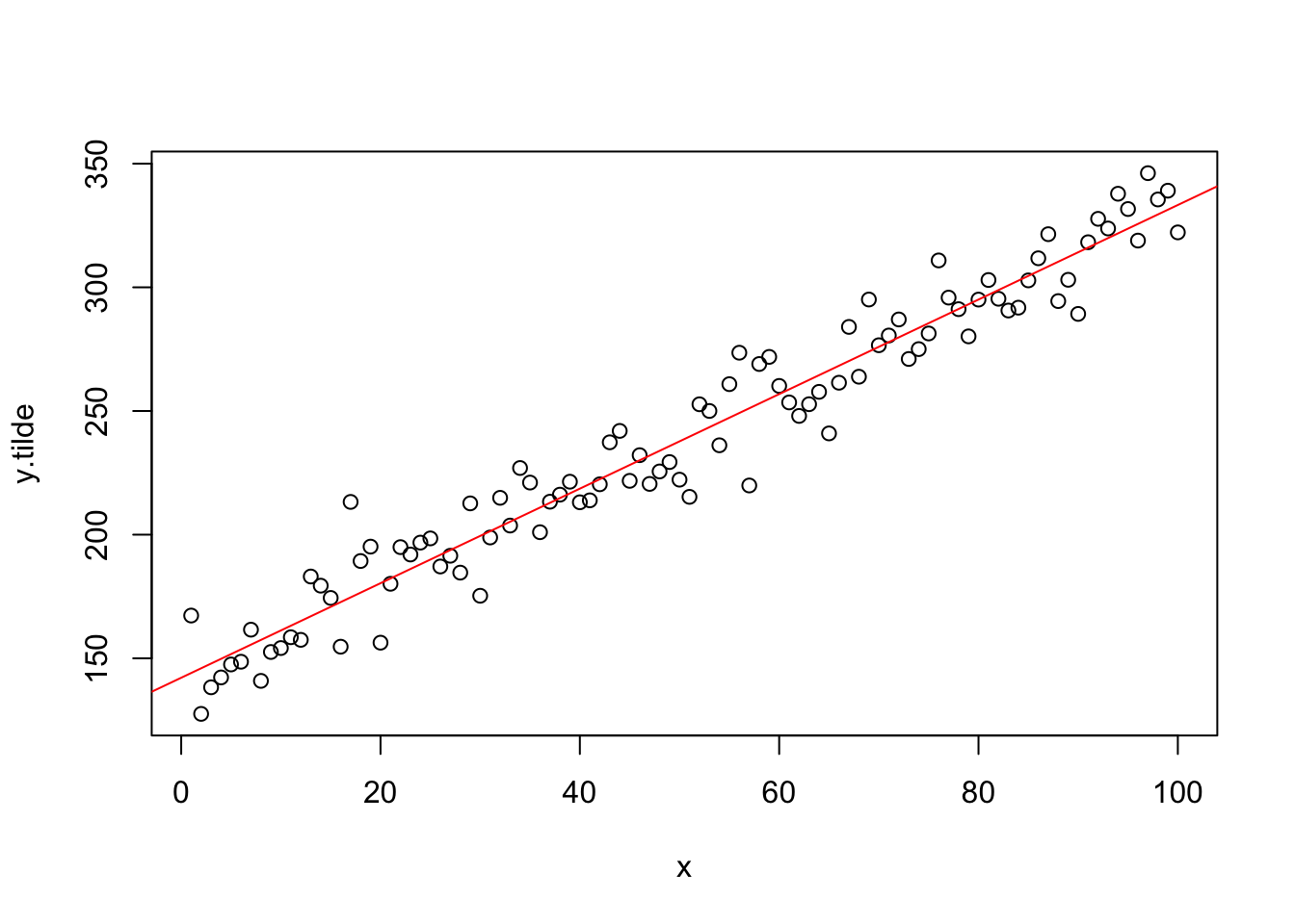

e.tilde=residuals(trans.model)
qqnorm(e.tilde)

shapiro.test(e.tilde)

## 
## 	Shapiro-Wilk normality test
## 
## data:  e.tilde
## W = 0.98912, p-value = 0.594

Using Transformed Model to Make Predictions

new.data=data.frame(x=runif(10,min=0,max=100))
y.tilde.hat=predict(trans.model,newdata=new.data)

plot(new.data$x,y.tilde.hat)
abline(trans.model,col="red")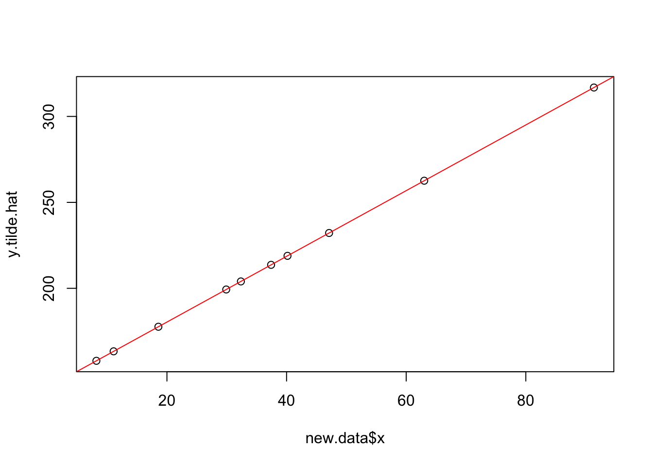

y.hat=y.tilde.hat^(1/lambda)

plot(x,y)
points(new.data$x,y.hat,col="red",pch=20)

4.2.4 Constancy of Error Variance (Homoscedasticity)

library("lawstat")


plot(x,abs(e))

levene.test(e,as.factor(x<=median(x)))

## 
## 	Modified robust Brown-Forsythe Levene-type test based on the absolute deviations from
## 	the median
## 
## data:  e
## Test Statistic = 7.3656, p-value = 0.007856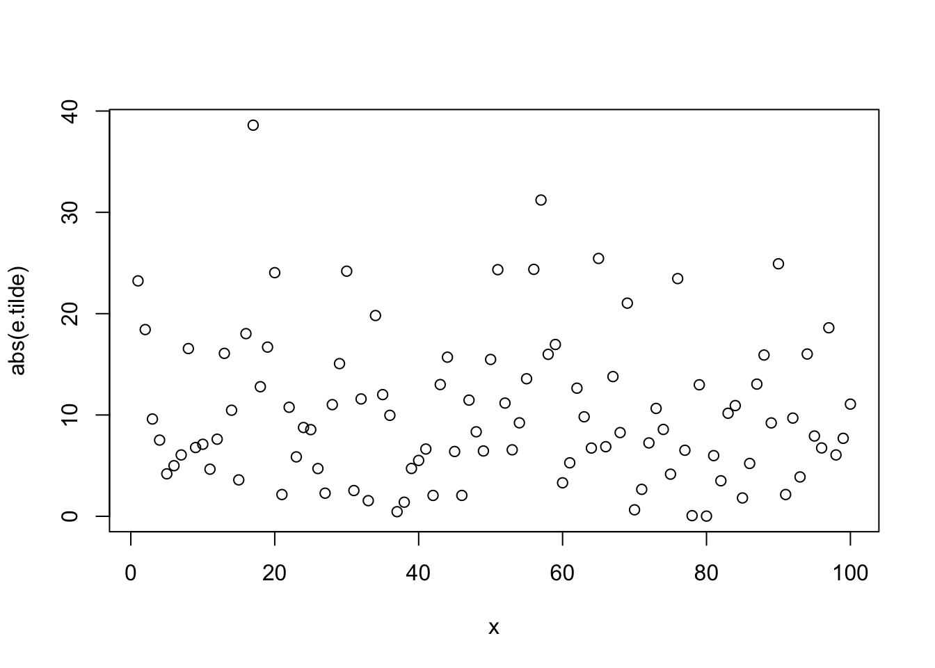

plot(x,abs(e.tilde))

levene.test(e.tilde,as.factor(x<=median(x)))

## 
## 	Modified robust Brown-Forsythe Levene-type test based on the absolute deviations from
## 	the median
## 
## data:  e.tilde
## Test Statistic = 0.24102, p-value = 0.6246

A Permutation Test Example

Creating Data

set.seed(403)
x1=runif(100,min=0,max=100)
x2=runif(100,min=0,max=100)
epsilon=runif(100,min=-50,max=50)

y=200+3*x1+5*x2+epsilon

mydata=data.frame(y,x1,x2)
plot(mydata)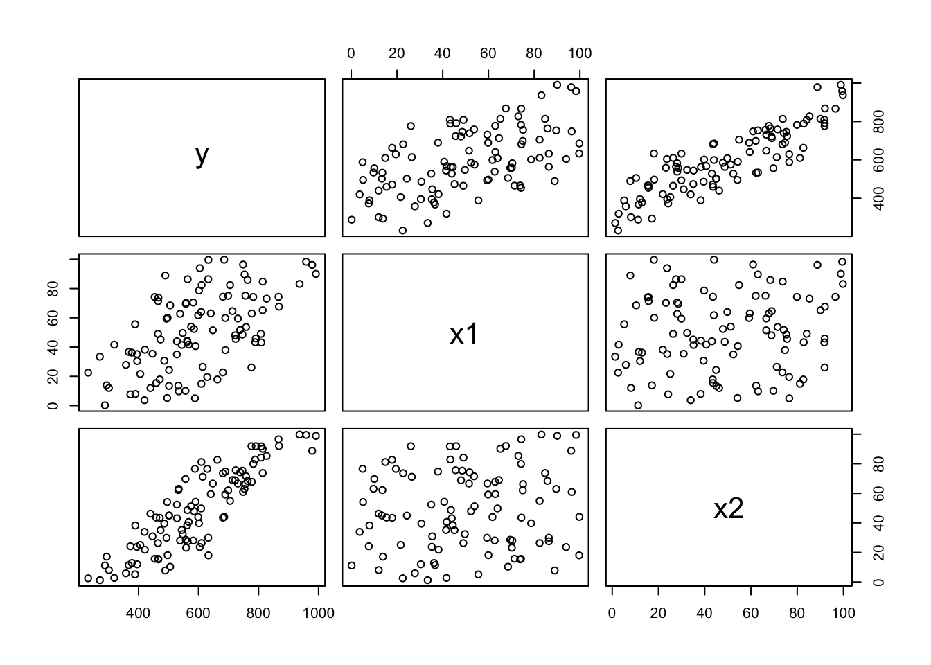

#Fitting a model and examining residuals
model=lm(y~x1+x2)
summary(model)

## 
## Call:
## lm(formula = y ~ x1 + x2)
## 
## Residuals:
##     Min      1Q  Median      3Q     Max 
## -51.954 -25.658  -3.725  26.312  54.757 
## 
## Coefficients:
##             Estimate Std. Error t value Pr(>|t|)    
## (Intercept) 206.5557     7.7986   26.49   <2e-16 ***
## x1            2.8750     0.1112   25.85   <2e-16 ***
## x2            4.9691     0.1091   45.53   <2e-16 ***
## ---
## Signif. codes:  0 '***' 0.001 '**' 0.01 '*' 0.05 '.' 0.1 ' ' 1
## 
## Residual standard error: 29.47 on 97 degrees of freedom
## Multiple R-squared:  0.9695,	Adjusted R-squared:  0.9689 
## F-statistic:  1543 on 2 and 97 DF,  p-value: < 2.2e-16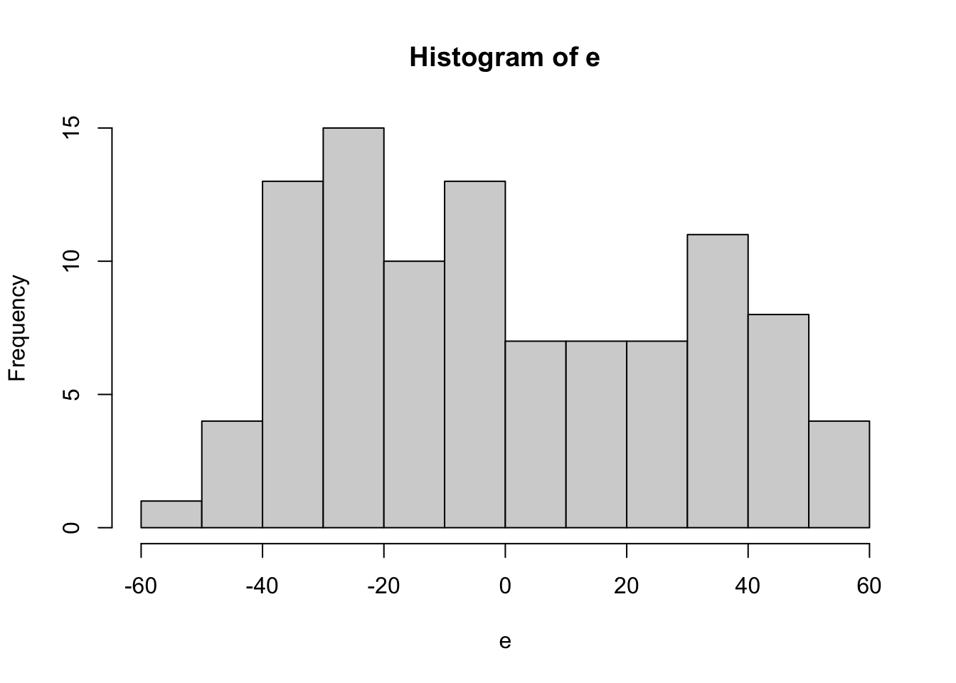

e=residuals(model)
hist(e)

qqnorm(e)

shapiro.test(e)

## 
## 	Shapiro-Wilk normality test
## 
## data:  e
## W = 0.94432, p-value = 0.000357

Model is y = beta0 + beta1*x1 + beta2*x2

Permutation Test for H0: beta2=0

N=1000
beta2.star.vect = 1:N


for(i in 1:N){
  temp.x2 = sample(x2,
                   size=length(x2),
                   replace=FALSE)
  temp.model=lm(y~x1+temp.x2)
  temp.betahat=coef(temp.model)
  beta2.star.vect[i]=temp.betahat[3]
}


hist(beta2.star.vect)     #All beta2 values from permutation test are stored in this vector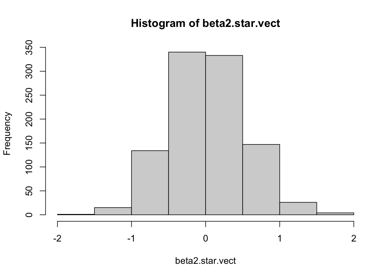

betahat=coef(model)

beta2hat=betahat[3]   
beta2hat                  #Actual value of beta2hat that we observed

##       x2 
## 4.969105

How do they compare?

range(beta2.star.vect)

## [1] -1.800433  1.622146

perm.pvalue=mean(abs(beta2hat)<=abs(beta2.star.vect))
perm.pvalue

## [1] 0