Chapter 3 Classification
3.0.1 Overview
This presentation covers the ways to create a machine learnining algorithm to classify cancerous cells. We will use differnt techniques and measure the accuracy of the prediction using each models.
The dataset comes from UCI Machine Learning Recipotary. You can read about the dataset in the website
Please note that this data is already cleaned and ready for use. So a majority of work is already done. Now we will use this data and predict if our algorithms can correctly classify.
what is being covered are as follows: – Decision Trees – KNN – Naive Bayes – Support Vector Machines – Artifitial Neural Networks
What is not being covered (will be covered separately) – Logistic Regression – Ensemble Methods – Other ML Algorithms – Cross Validation – Changing Default parameters and tuning models
3.0.2 Getting the data
Download the data direcelty from the source to R. Please get acquinted with the data and the variable names. The following code chunk saves the data in the R environment as wdbc and provides the column name that we assign to it.
#the dataset does not have headers and is a comma seperated dataset

link <- "http://archive.ics.uci.edu/ml/machine-learning-databases/breast-cancer-wisconsin/wdbc.data"

col_names<- c("id", "diagnosis", "radius_1", "texture_1", "perim_1", "area_1", "smooth_1", "compact_1", "concavity_1", "concave_pts_1", "symmetry_1", "frac_dim_1",
              "radius_2", "texture_2", "perim_2", "area_2", "smooth_2", "compact_2", "concavity_2", "concave_pts_2", "symmetry_2", "frac_dim_2",
              "radius_3", "texture_3", "perim_3", "area_3", "smooth_3", "compact_3", "concavity_3", "concave_pts_3", "symmetry_3", "frac_dim_3"          )

wdbc<- read.table(url(link), header = F, sep = ',', col.names = col_names)
Once the data is loaded to the R environment, it is import to explore it to understand the data itself. The results of following codes are hidden.
head(wdbc, 5)   #shows us first 5 data, default is 6
tail(wdbc, 10)  #opposite of head
summary(wdbc)   #gives the five number summary for each quantitative variable
names(wdbc)     #the column names we assigned
str(wdbc)
These gives the basic idea of how the data are. From str(wdbc) it can be seen that all the variables are numerical and diagnosis is categorical with two levels, M and B. And our goal here will be to predict diagnosis based on other variables.
After some thought we realize that the column id is not necessary. So we remove it. Also remember that there are each cell nucleus is measured three different times using different methods (mean, standard error, and worst).
The scatter Matrix below shows how each variables are related to other
##   radius_1 radius_2 radius_3
## 1 17.99 1.095 25.38pairs(wdbc[,2:11], upper.panel = NULL, col= c("red", "green")[wdbc$diagnosis],
main ="Scatterplot matrix of wdbc dataset \n measurements method 1") Notice that now there are only 31 columns now.
3.0.3 Exploring dataset using statistics and plots (ggplot2)
A lot can be realized about the data through simple statistics and plots of the data. It is up to an individual data anaylst on how they want to explore the data before they start making the model. Following are a few ways data can be explored. Play with different built in functions and plots.
##
##   B   M
## 357 212##
## B M
## 0.6274165 0.3725835##
## B M
## FALSE 0.147627417 0.001757469
## TRUE 0.479789104 0.370826011## wdbc$diagnosis: B
## Min. 1st Qu. Median Mean 3rd Qu. Max.
## 6.981 11.080 12.200 12.147 13.370 17.850
## ---------------------------------------------------------------------------
## wdbc$diagnosis: M
## Min. 1st Qu. Median Mean 3rd Qu. Max.
## 10.95 15.07 17.32 17.46 19.59 28.11Can we say that malignant cells have bigger radius than benign cells?
3.0.4 Quick tutorial of plotting in ggplot2
It is time to install and load ggplot2 library
library(ggplot2)
#plotting scatterplots of two points and adding smooth line
ggplot(aes(x = radius_1, y = area_1), data = wdbc)+
  geom_point()+geom_smooth()
## `geom_smooth()` using method = 'loess' and formula 'y ~ x'
## [1] 0.9873572#histogram of texture_1 where diagnosis = B
ggplot(aes(x= texture_1), data = subset(wdbc, diagnosis =="B"))+
geom_histogram(binwidth =2, color =I("Black"))
#plotting two line graph from histogram
ggplot(aes(x= texture_1), data = wdbc)+ geom_freqpoly(binwidth =1)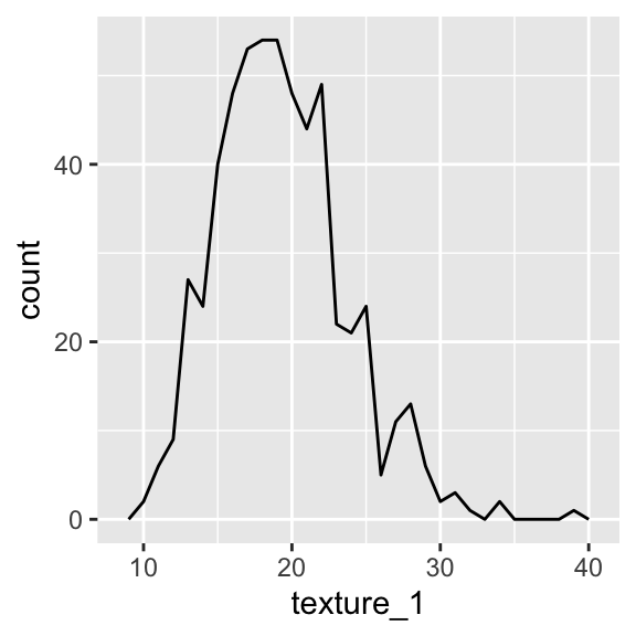
#plotting bunch on of two variable things in one plot
ggplot(aes(x = area_1, y = texture_1), data = wdbc)+geom_line()+geom_point()+geom_smooth()
## `geom_smooth()` using method = 'loess' and formula 'y ~ x'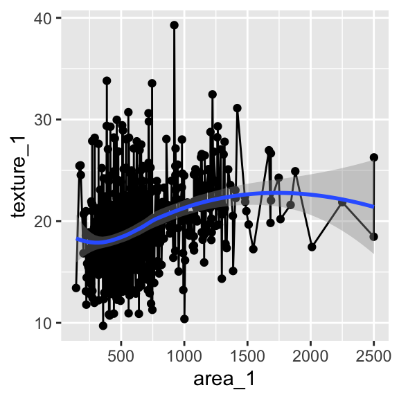
#plotting boxplots
ggplot(aes(x =diagnosis, y = frac_dim_1, color = I("red"), fill = I("blue")),data = wdbc) +
  geom_boxplot()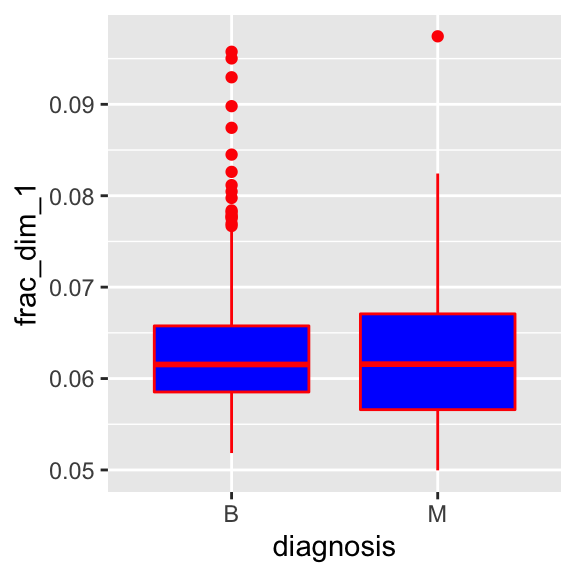
#comparing same variable for two classes by faceting
ggplot(aes(x =texture_1), data = wdbc)+geom_freqpoly(binwidth = 1) +facet_wrap(~diagnosis)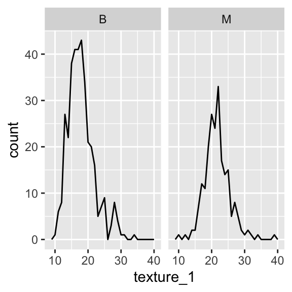
There is much more to it. Note that base R plot functions can also produce similar. Best way to learn exploratory data analysis through ggplot is to ask interesting questions and try to plot it and see if you hypothesis comes true or not.
3.1 Building our Machine Learning Algorithm
This will briefly cover some Machine Learning algorithm and how they can be used in making prediction. This will however not cover how to improve the models, change default parameters, doing cross validations and creating confusion matrices and using it to find the accuracy and error rates. They will be covered in the future.
We have aready created the most fundamental models. It is just simple guess and check method. Earlier we tabulated how many of the cells had radius >11 and which category they belonged to. That is a simple predictive model. However things are not always simple and they are affected by more than one variable. Machine Learning Algorithms help in such cases. Here are some algorithms that are widely used.
3.1 Decision Trees
We will be using decision trees to classify the cells into M or B based on other variables. For theories on decision tree please read the textbook or this [Wikipedia entry] (https://en.wikipedia.org/wiki/Decision_tree)
Install and load the following rpart, rpart.plot and rattle libraries
library(rpart)
library(rattle)
library(rpart.plot)

#first decision tree model
first_dt<- rpart(diagnosis~., data = wdbc) #using all columns of wdbc as independent variables
first_dt
## n= 569
##
## node), split, n, loss, yval, (yprob)
## * denotes terminal node
##
## 1) root 569 212 B (0.62741652 0.37258348)
## 2) radius_3< 16.795 379 33 B (0.91292876 0.08707124)
## 4) concave_pts_3< 0.1358 333 5 B (0.98498498 0.01501502) *
## 5) concave_pts_3>=0.1358 46 18 M (0.39130435 0.60869565)
## 10) texture_3< 25.67 19 4 B (0.78947368 0.21052632) *
## 11) texture_3>=25.67 27 3 M (0.11111111 0.88888889) *
## 3) radius_3>=16.795 190 11 M (0.05789474 0.94210526) *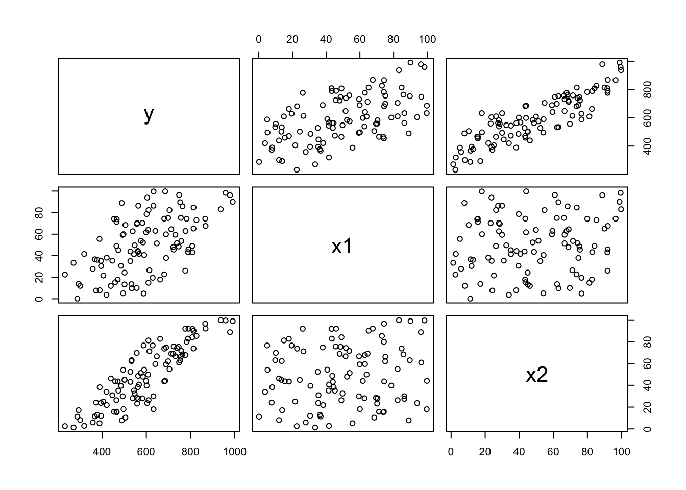
You can enter the code summary(first_dt) to see mathematical output of decision trees. In this example, we fed in all the data we had in the model. This gives us the output but this is not what we are looking for. This is called overfitting. We want to create a model so that when we feed in newer data, the model predicts the output for this data correctly.
To train our model, we will need to divide our dataset into two sets, training and testing sets. We will use training data to train the model and then test the validity of the model using the testing data.
#setting seed so that the process is replicable with same results
set.seed(445)

#taking sample of rows, 70%, of wdbc data
sample_rows.wdbc<- sample(nrow(wdbc), round(.7*nrow(wdbc), 0))

train.wdbc<- wdbc[sample_rows.wdbc, ] #subsetting wdbc using sample from code above
test.wdbc<- wdbc[-sample_rows.wdbc, ] # -sample_rows.wdbc finds the rows that was not sampled

dim(wdbc)
## [1] 569 31## [1] 398 31## [1] TRUESo, now we have splitted the wdbc dataset into two separate dataset in no particular order. We can now build the model using training data and test using testing data
wdbc.tree_1 <- rpart(diagnosis~., data = train.wdbc) #we are using default parameters

#predicting the outcome using our model above
predict.tree_1<- predict(wdbc.tree_1, newdata = test.wdbc, type = "class")
table(predict.tree_1)
## predict.tree_1
## B M
## 113 58So, we predicted diagnosis results on testing set using the model we created by using training dataset. How do we know if our prediction is correct. Well, in this case we compare the result from our model against the true value in the test data.
##
## predict.tree_1   B   M
##              B 101  12
##              M   1  57
Decision tree was a very easy solution to this problem because it recognized the important factors for the diagnosis in three splits with accuracy 0.9239766.
Will model predict as good if the data was sampled in different ways? In order to do that, we need to engineer the features and reduce overfitting. A simpler model that predicts well over longer term is a better model than a more complex model that only perfoms on certain data. We can also play with the tree default parameters. We will skip feature engineering and cross validation for now.
3.1 Kth- Nearest Neighbours (KNN)
In Layman’s term, in KNN algorithm, the test data point finds the closest neighbour from the train data. The idea is that items with similar features live closer to each other.
library(class)
# removing the categorical variables from both test and train dataset and telling knn to learn from diagnostics column from training dataset
wdbc.knn_1 <- knn(train = train.wdbc[, -1], test = test.wdbc[,-1], cl = train.wdbc$diagnosis, k = 5)

table(wdbc.knn_1, test.wdbc$diagnosis)
##
## wdbc.knn_1 B M
## B 98 10
## M 4 59This KNN model found the nearest 5 neighbours of the test point and classified it into whichever set B or M had at least 3 training set into it. The accuracy of prediction is 0.9181287
We did not normalize the data in this example. Normalization like Z score from X is necessary. Also , feature engineering and cross validation is skipped for now.
We will also use kknn package in the future and see the power of Kth- Nearest Neighbour algorighm.
3.1 Naive Bayes
Naive Bayes classifier algorithm is the closest to the Baysian Model and it relies on probability of events happening prior. If you remember conditional probabilities from statistics, you are making good progress.
Install and load e1071 library
library(e1071)
wdbc.naive_1<- naiveBayes(diagnosis ~ .,data = train.wdbc)

predict.naive_1<- predict(wdbc.naive_1, newdata = test.wdbc[,-1])
print(predict.naive_1)
## factor(0)
## Levels:With the basic naive bayes model we got the accuracy of 0.9181287
Again, there is a lot of optimization we can do using this method which is skipped here for now.
3.1 Support Vector Machines
SVM is a very powerful techniques whose workings consists of applied math (linear algebra).
Install and load e1071 library
# wdbc.svm_1<- svm(diagnosis~., data = train.wdbc)
#
# predict.svm_1<- predict(wdbc.svm_1, newdata = test.wdbc[-1])
#
# table(predict.svm_1, test.wdbc$diagnosis)
This algorithm used the default linear separator/kernel with reasonable cost. The parameter of SVM must be tuned to get sensible results. However this model predicted very successfully at the rate of 0.9649123
3.1 Artifitial Neural Netrowks
Artifitial Neural Networks algorithm closely resemble the neurons or workings of brains. It consists of one input and output layer and multiple hidden ones.
Install and load the nnet library
library(nnet)

# wdbc.nnet_1 <- nnet(diagnosis~., data =  train.wdbc, size = 8)
# predict.nnet_1<- predict(wdbc.nnet_1, newdata = test.wdbc[-1], type ="class")
#
# table(predict.nnet_1, test.wdbc$diagnosis)
The artificial neural network algorithm on this data had the accuracy of 0.9239766