Chapter 2 Statistics for Data Science

We will skip the introductory statistics. There are many courses/ textbook out there. Recommended coursebook:

Mean, Median, Mode, Variance, Standard Deviation
Sample, Population
Expected values, Estimation
Probability
Permutations and Combinations
Distributions (Binomial, Normal, Poisson, Hypergeometric, etc.)
Test Statistic and statistical inference (Z-test, T-Test, Confidence interval, etc.)
Hypothesis Testing

R is equipped with many statistical functions. We can calculate metrics such mean, mean, median, mean, max, etc. of the given vector using functions in R.

x=rnorm(1000,100,15)  #Generates a sample of size 1000 from a normal distribution with mu=100 and sigma=15

mean_x = mean(x)   #Computes the sample mean.
sd_x = sd(x)     #Computes the sample st dev.

sum_x = sum(x)    #Computes the sum of the elements of x.

print(paste0("mean_x = ", mean_x, " sd_x = ", sd_x, " sum_x = ", sum_x))

## [1] "mean_x = 100.328393193161 sd_x = 14.5746365457083 sum_x = 100328.393193161"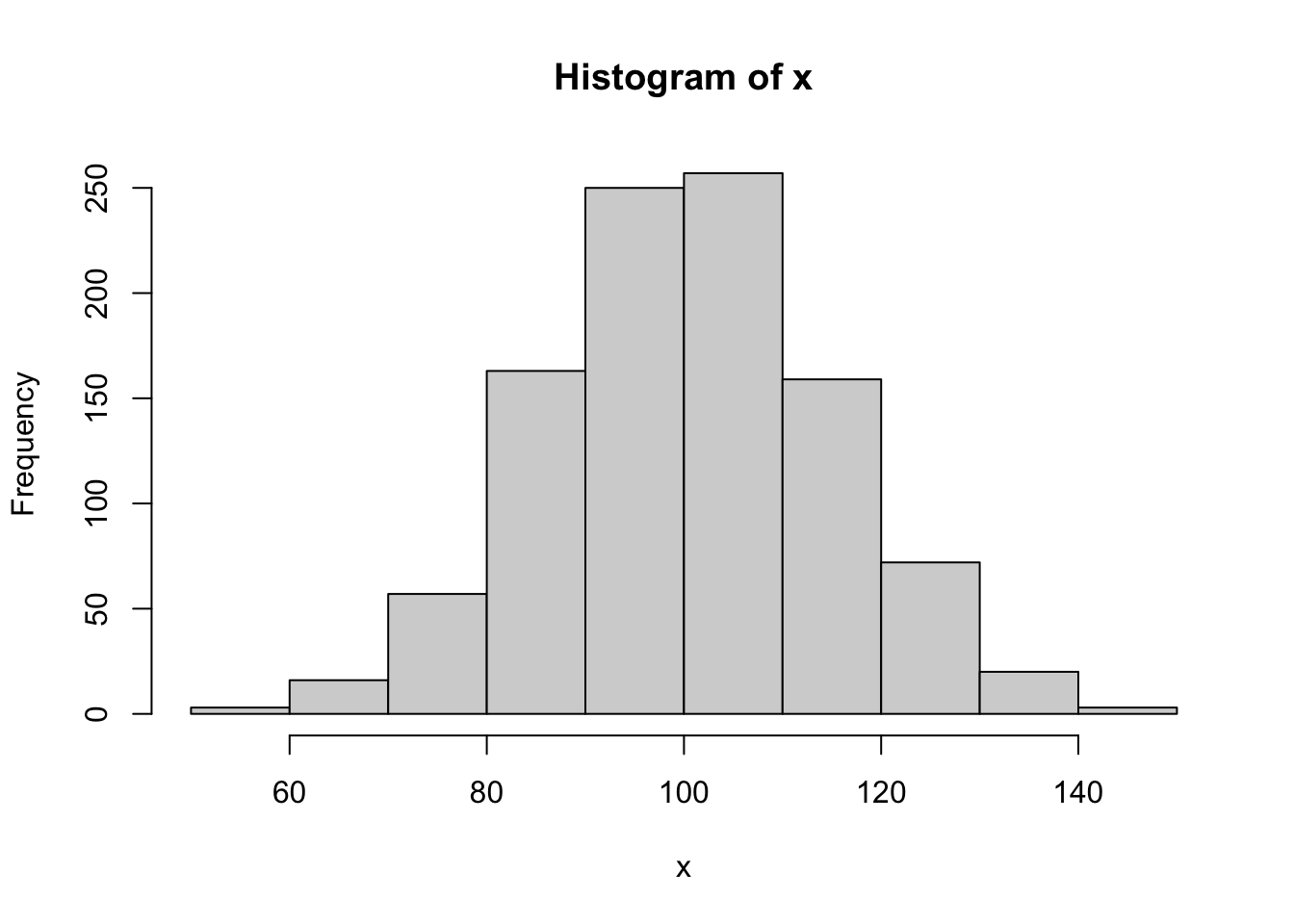

hist(x)   #Plots a histogram for x.

u=runif(1000,10,20)  #Generates a sample of size 1000 from a uniform
                     #Distribution on the interval [10,20].

min_u = min(u)    #Finds the smallest component of u.
max_u = max(u)    #Finds the largest component of u.

sorted_u=sort(u)
length(sorted_u)

## [1] 1000

sorted_u[1]

## [1] 10.01506

sorted_u[1000]

## [1] 19.99784

x=rnorm(1000,100,15)       #Random x values.
epsilon=rnorm(1000,0,5)    #Random "errors".
y=x+epsilon                #Random y values dependent on x.

plot(x,y)                  #Scatterplot of (x,y) pairs.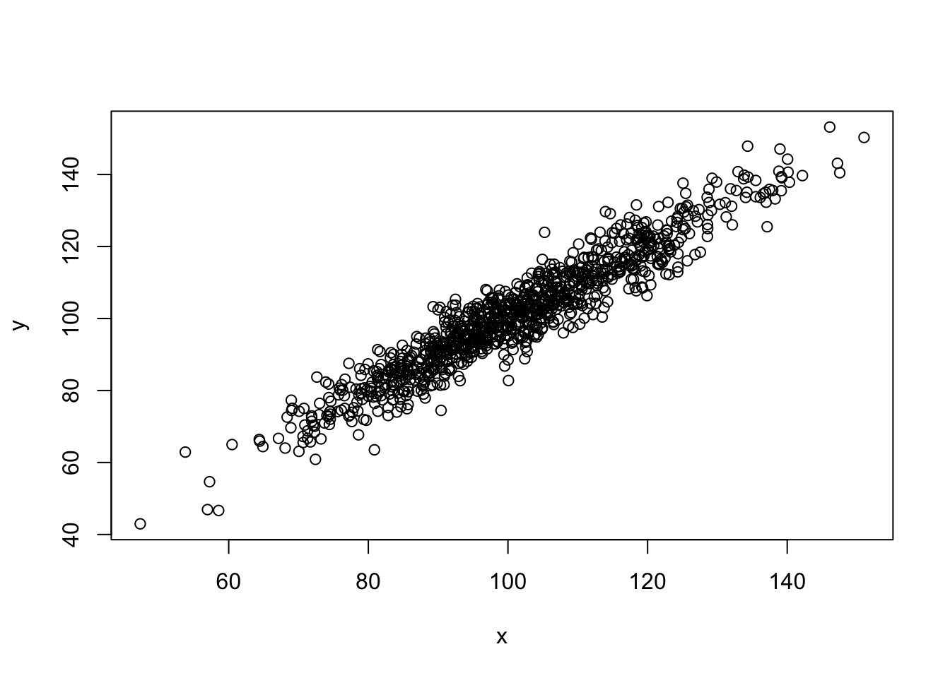

plot(-10:10,(-10:10)^2)    #Plot of the parabola y=x^2.

plot(-10:10,(-10:10)^2,type='l')

2.1 Non Parametric Statistics

Parametric statistics are the ones where we know the behavior of the population. Usually the parameters of a statistical methods are the mean and the standard deviation. Eg. confidence interval

In contrast, in non-parametrc statistics we do not need to make any assumption about the population. Non parametric methods are easy to use and apply. Refer to Conover Practical Nonparametric statistics

2.1.1 Sign Test and variations

Use to test if preferance A vs B

Number of response with positive preferance \([num\ +]\)
Number of response with negative preferance \([num\ -\)
Number of response with no preferance. We do not care for those
We test the hypothesis that:
- \(H_0: P(+) = P(-)\ vs\ H_1: P(+) ! = P(_)\)
- with \(n = [num \ +] + [num \ -]\)
- and test statistic \(T = [num \ +]\)
- Null Distribution \(T \~ B(n, 0.5)\)

McNemar Test of Significant Changes (sign test variant)

Eg: differenct between voter intentions before and after debate

Cox-Stuart Test for Trend (sign test variant)

Eg. Given the temperature for last 19 January Check if trend in temperature pattern exists. (hint: convert the temp between two consecutive January to + or - based on pattern and count those up)

2.1.2 chi squared tests for contengency tables

2.1.3 Median test

To test whether the sample median is different from grand median (population median)

2.1.4 Measure of Dependence

2.1.5 Chi-Squared goodness of fit tests

2.1.7 Mann - Whitney - Wilcoxin Test

Tests if two samples are independent.

Assumes that two samples are from different population.
Assumes that samples are statistically independent of each other
Measurement scale is at least ordinal
Null Hypothesis: Two probability distributions are identitcal
Rank observations from smallest to largest
Test Statistic \(T = \sum _{i=1}^{n} Rank(X_i)\)

Steps:

sort the values
Assign Rank
Replace Ties
Calcualte T
Calculate W

#Example:  Farm Boys and Town Boys

#Creating data set
residence=c(rep("Farm",12),rep("Town",36))
residence=as.factor(residence)
fitness=c(c(14.8,7.3,5.6,6.3,9.0,4.2),
          c(10.6,12.5,12.9,16.1,11.4,2.7),
          c(12.7,14.2,12.6,2.1,17.7,11.8),
          c(16.9,7.9,16.0,10.6,5.6,5.6),
          c(7.6,11.3,8.3,6.7,3.6,1.0),
          c(2.4,6.4,9.1,6.7,18.6,3.2),
          c(6.2,6.1,15.3,10.6,1.8,5.9),
          c(9.9,10.6,14.8,5.0,2.6,4.0))
mydata=data.frame(residence,fitness)


#Mann-Whitney-Wilcoxon Test
wilcox.test(fitness~residence,data=mydata)

## Warning in wilcox.test.default(x = c(14.8, 7.3, 5.6, 6.3, 9, 4.2, 10.6, : cannot compute exact p-
## value with ties

## 
## 	Wilcoxon rank sum test with continuity correction
## 
## data:  fitness by residence
## W = 243, p-value = 0.5279
## alternative hypothesis: true location shift is not equal to 0

Calculating Wilcoxin (mann-whitney-wilcoxin) Test

#Sort the data
mydata=mydata[order(mydata$fitness),]

#Assigning ranks
dim(mydata)

## [1] 48  2

mydata=cbind(mydata,rank=1:48)

#Replacing ties 
mydata$rank[12:14]=13
mydata$rank[20:21]=20.5
mydata$rank[29:32]=30.5
mydata$rank[41:42]=41.5

#Calculating T
T_value = sum(mydata$rank[mydata$residence=="Farm"])
T_value

## [1] 321

#Calculating W
W_val = T_value -12*(12+1)/2
W_val

## [1] 243

2.1.8 Kruskal-Wallis Test

Use it for Several Independent Samples. Extends mann-whitney-wilcoxin test for more than two samples using same assumptions and hypothesis

#Example:  Corn Yields
corn.yield=c(c(83,91,94,89,89,96,91,92,90),
             c(91,90,81,83,84,83,88,91,89,84),
             c(101,100,91,93,96,95,94),
             c(78,82,81,77,79,81,80,81))
farming.method=as.factor(c(rep(1,9),
                           rep(2,10),
                           rep(3,7),
                           rep(4,8)))
mydata2=data.frame(corn.yield,farming.method)


#Plot of data
plot(farming.method,corn.yield,data=mydata2)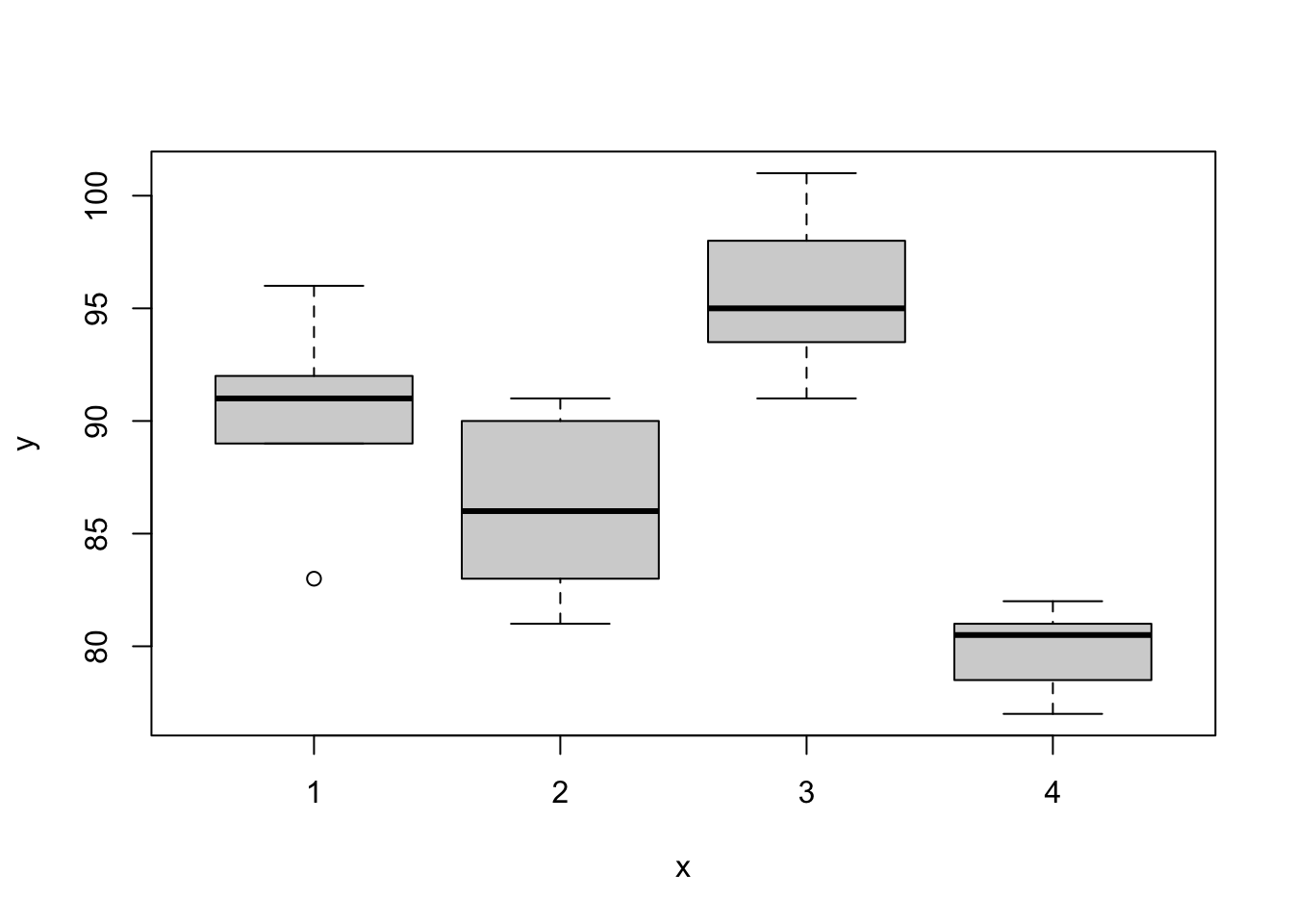

#Kruskal-Wallis Test
kruskal.test(corn.yield~farming.method,data=mydata2)

## 
## 	Kruskal-Wallis rank sum test
## 
## data:  corn.yield by farming.method
## Kruskal-Wallis chi-squared = 25.629, df = 3, p-value = 1.141e-05

kruskal.test(fitness~residence,data=mydata)

## 
## 	Kruskal-Wallis rank sum test
## 
## data:  fitness by residence
## Kruskal-Wallis chi-squared = 0.41362, df = 1, p-value = 0.5201

2.1.9 Wilcoxin-signed-rank Test

For matched pairs

Random sample of pairs
Null Hypothesis that exepcted value of two samples are same
Discard ties and calculate absolute difference (since difference between the pairs is 0)

Steps:

Calculate differences
Discard ties
Sort data based on absolute differences
Create Rank
Replace ties
Create Signed Ranks
Calculate R
Calculate Tplus
Run mann-whitney-wilcox test

#Example:  Twins
firstborn=c(86,71,77,68,91,72,77,91,70,71,88,87)
secondborn=c(88,77,76,64,96,72,65,90,65,80,81,72)

#Wilcox Signed Ranks Test
wilcox.test(secondborn,firstborn,paired=TRUE)

## Warning in wilcox.test.default(secondborn, firstborn, paired = TRUE): cannot compute exact p-value
## with ties

## Warning in wilcox.test.default(secondborn, firstborn, paired = TRUE): cannot compute exact p-value
## with zeroes

## 
## 	Wilcoxon signed rank test with continuity correction
## 
## data:  secondborn and firstborn
## V = 24.5, p-value = 0.4765
## alternative hypothesis: true location shift is not equal to 0

Step by step exapmple

#Calculating differences
mydata3=data.frame(firstborn,
                   secondborn,
                   D=secondborn-firstborn,
                   absD=abs(secondborn-firstborn))

#Discarding ties
mydata3=mydata3[mydata3$D!=0,]

#Sort data based on absD
mydata3=mydata3[order(mydata3$absD),]

#Creating absD ranks
mydata3=cbind(mydata3,absD.rank=1:11)

#Replacing absD rank ties
mydata3$absD.rank[1:2]=1.5
mydata3$absD.rank[5:6]=5.5

#Creating signed ranks R
R=(mydata3$absD.rank)*sign(mydata3$D)
mydata3=cbind(mydata3,R)

#Calculating Tplus
Tplus=sum(R[R>0])
Tplus

## [1] 24.5

wilcox.test(secondborn,firstborn,paired=TRUE)

## Warning in wilcox.test.default(secondborn, firstborn, paired = TRUE): cannot compute exact p-value
## with ties

## Warning in wilcox.test.default(secondborn, firstborn, paired = TRUE): cannot compute exact p-value
## with zeroes

## 
## 	Wilcoxon signed rank test with continuity correction
## 
## data:  secondborn and firstborn
## V = 24.5, p-value = 0.4765
## alternative hypothesis: true location shift is not equal to 0

#Switching the order
wilcox.test(firstborn,secondborn,paired=TRUE)

## Warning in wilcox.test.default(firstborn, secondborn, paired = TRUE): cannot compute exact p-value
## with ties

## Warning in wilcox.test.default(firstborn, secondborn, paired = TRUE): cannot compute exact p-value
## with zeroes

## 
## 	Wilcoxon signed rank test with continuity correction
## 
## data:  firstborn and secondborn
## V = 41.5, p-value = 0.4765
## alternative hypothesis: true location shift is not equal to 0

sum(R[R<0])

## [1] -41.5

2.1.10 Quade Test

For Several Related Samples

#Example:  Hand Lotion Sales
y <- matrix(c( 5,  4,  7, 10, 12,
               1,  3,  1,  0,  2,
               16, 12, 22, 22, 35,
               5,  4,  3,  5,  4,
               10,  9,  7, 13, 10,
               19, 18, 28, 37, 58,
               10,  7,  6,  8,  7),
            nrow = 7, byrow = TRUE,
            dimnames =
              list(Store = as.character(1:7),
                   Brand = LETTERS[1:5]))

y

##      Brand
## Store  A  B  C  D  E
##     1  5  4  7 10 12
##     2  1  3  1  0  2
##     3 16 12 22 22 35
##     4  5  4  3  5  4
##     5 10  9  7 13 10
##     6 19 18 28 37 58
##     7 10  7  6  8  7

#Quade Test
quade.test(y)

## 
## 	Quade test
## 
## data:  y
## Quade F = 3.8293, num df = 4, denom df = 24, p-value = 0.01519

2.1.11 Spearman’s Test

Measures of rank correlation

#Two independent samples
x=rnorm(1000)
y=rnorm(1000)
plot(x,y)

#Correlations
cor(x,y)

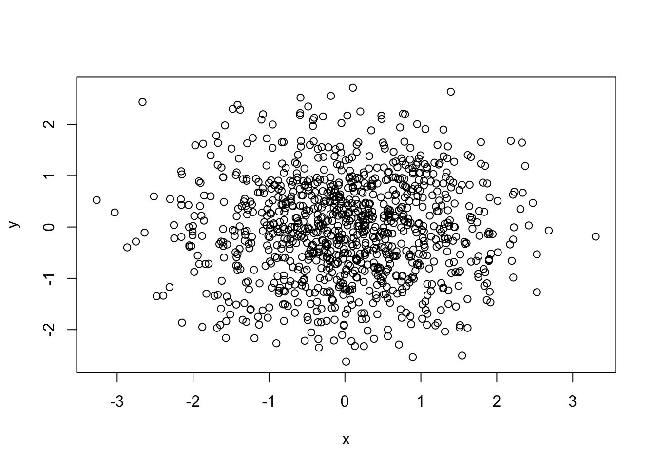
## [1] -0.005149681

cor(x,y,method="spearman")

## [1] 0.0004317244

#Correlation tests
#Null hypothesis is that x and y are uncorrelated.
cor.test(x,y)

## 
## 	Pearson's product-moment correlation
## 
## data:  x and y
## t = -0.16269, df = 998, p-value = 0.8708
## alternative hypothesis: true correlation is not equal to 0
## 95 percent confidence interval:
##  -0.06712134  0.05686155
## sample estimates:
##          cor 
## -0.005149681

cor.test(x,y,method="spearman")

## 
## 	Spearman's rank correlation rho
## 
## data:  x and y
## S = 166594546, p-value = 0.9891
## alternative hypothesis: true rho is not equal to 0
## sample estimates:
##          rho 
## 0.0004317244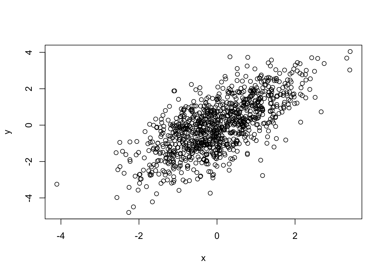

#Two dependent samples
x=rnorm(1000)
y=x+rnorm(1000)
plot(x,y)

#Correlations
cor(x,y)

## [1] 0.6901655

cor(x,y,method="spearman")

## [1] 0.6645341

#Correlation tests
#Null hypothesis is that x and y are uncorrelated.
cor.test(x,y)

## 
## 	Pearson's product-moment correlation
## 
## data:  x and y
## t = 30.129, df = 998, p-value < 2.2e-16
## alternative hypothesis: true correlation is not equal to 0
## 95 percent confidence interval:
##  0.6562504 0.7212975
## sample estimates:
##       cor 
## 0.6901655

cor.test(x,y,method="spearman")

## 
## 	Spearman's rank correlation rho
## 
## data:  x and y
## S = 55910934, p-value < 2.2e-16
## alternative hypothesis: true rho is not equal to 0
## sample estimates:
##       rho 
## 0.6645341

2.1.12 Assessing Normality

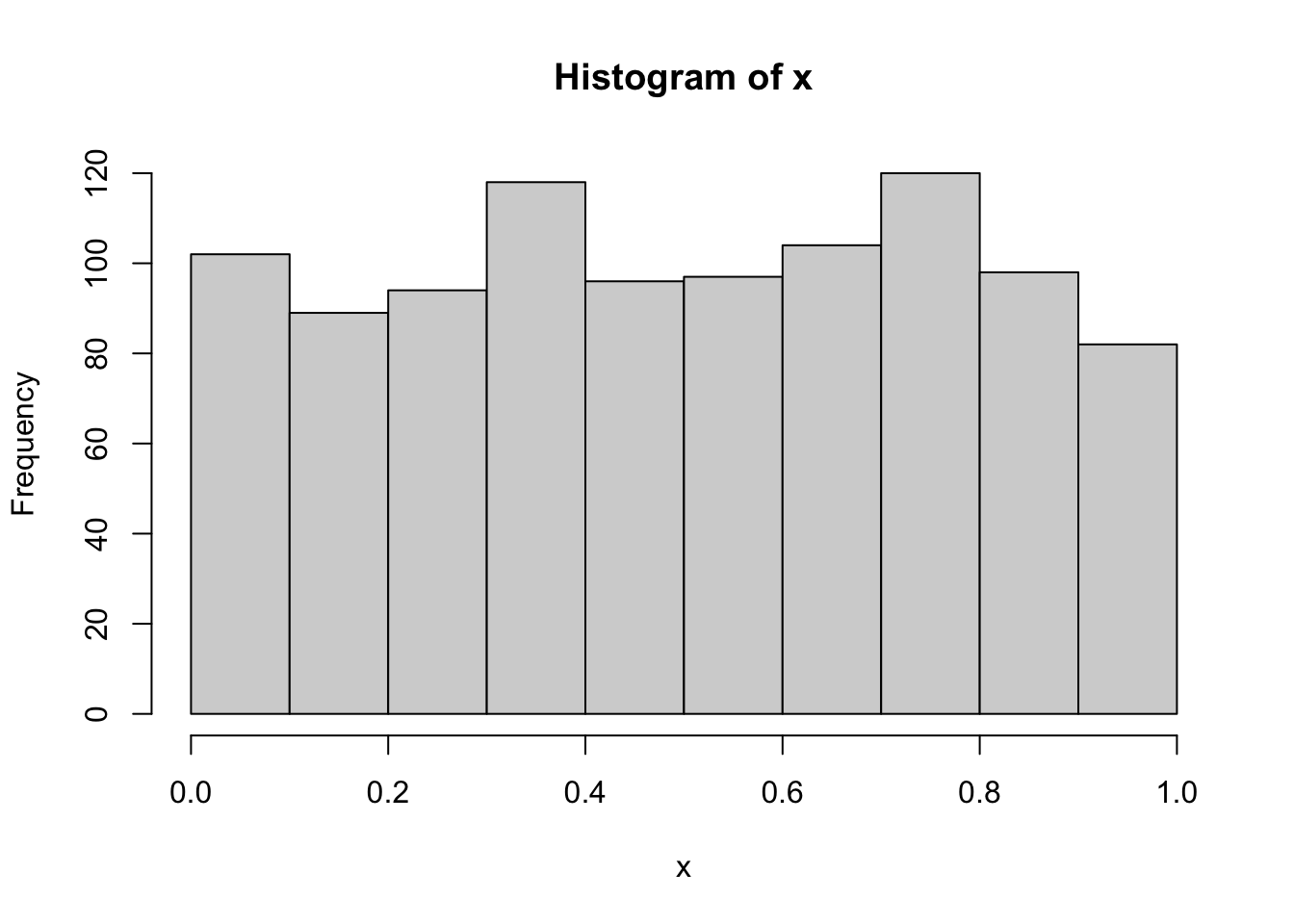
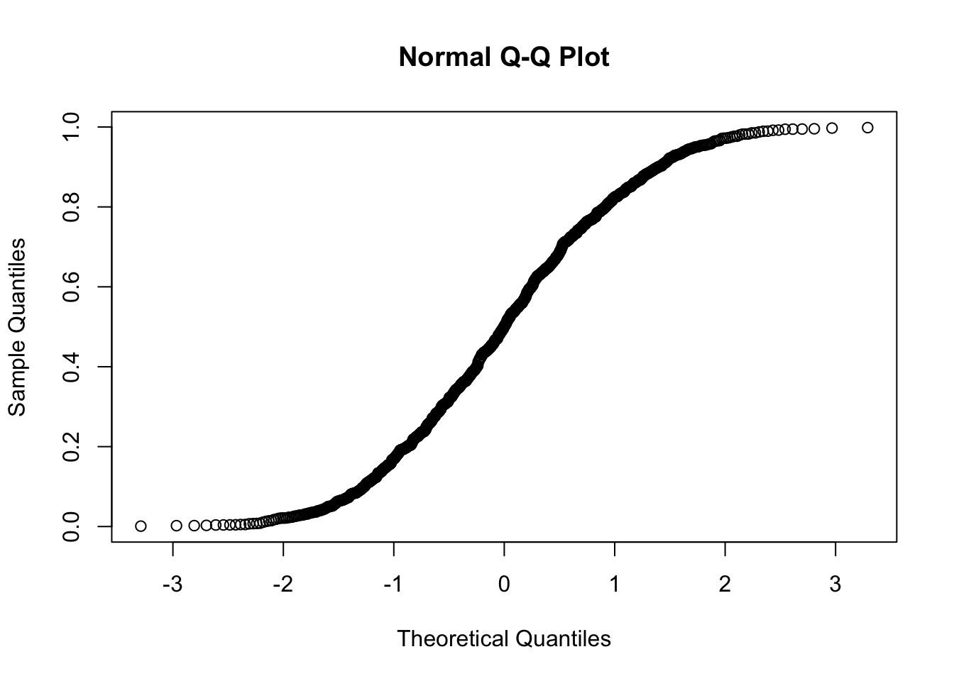
Using quantile-quantile-plots and Hypothesis Tests

#Example 1:  Normal data
x=rnorm(1000)
qqnorm(x)

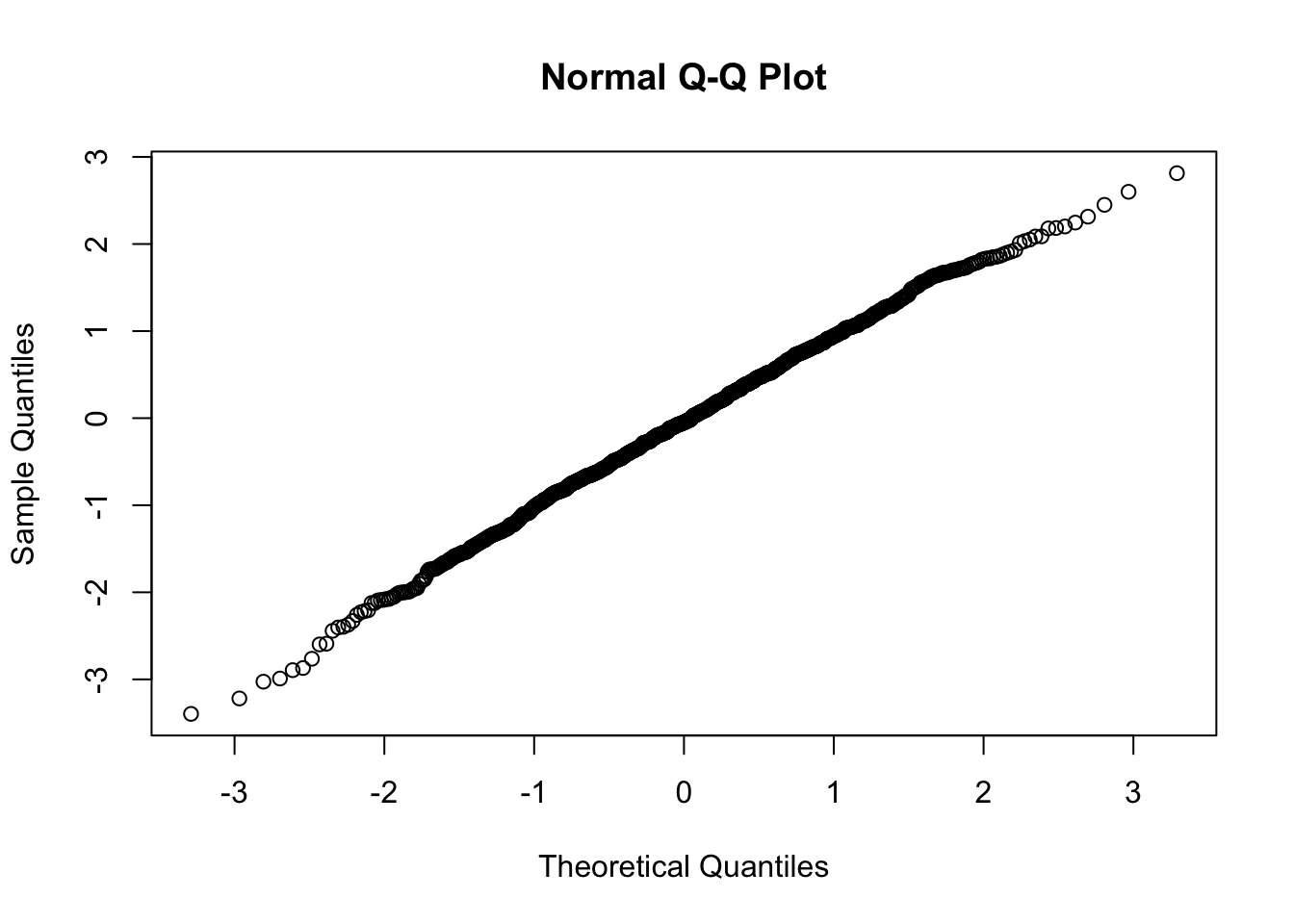
Using Kolmogorov-Smirnov Test

#Null hypothesis is that x and y have the same distribution
ks.test(x,y="pnorm")

## 
## 	One-sample Kolmogorov-Smirnov test
## 
## data:  x
## D = 0.024585, p-value = 0.5812
## alternative hypothesis: two-sided

Using Shapiro-Wilk Test.

#Null hypothsis is that x is normally distributed
shapiro.test(x)

## 
## 	Shapiro-Wilk normality test
## 
## data:  x
## W = 0.99753, p-value = 0.1367

Normality example using all methods explained

#Example 2:  Uniform data
x=runif(1000)
hist(x)

qqnorm(x)

#Kolmogorov-Smirnov Test
#Null hypothesis is that x and y have the same distribution
ks.test(x,y="pnorm")

## 
## 	One-sample Kolmogorov-Smirnov test
## 
## data:  x
## D = 0.5004, p-value < 2.2e-16
## alternative hypothesis: two-sided

ks.test(x,y="punif")

## 
## 	One-sample Kolmogorov-Smirnov test
## 
## data:  x
## D = 0.024197, p-value = 0.6017
## alternative hypothesis: two-sided

#Shapiro-Wilk Test.
#Null hypothsis is that x is normally distributed
shapiro.test(x)

## 
## 	Shapiro-Wilk normality test
## 
## data:  x
## W = 0.95951, p-value = 5.12e-16