Chapter 5 Logistic Regression
5.0.1 Simple Example
Generating data
Estimating model coefficients
##
## Call:
## glm(formula = Y ~ X, family = binomial)
##
## Deviance Residuals:
##     Min       1Q   Median       3Q      Max
## -2.4713  -0.6868  -0.3107   0.6862   2.4725
##
## Coefficients:
##               Estimate Std. Error z value Pr(>|z|)
## (Intercept) -3.0096470  0.0198147  -151.9   <2e-16 ***
## X            0.0601529  0.0003612   166.5   <2e-16 ***
## ---
## Signif. codes:  0 '***' 0.001 '**' 0.01 '*' 0.05 '.' 0.1 ' ' 1
##
## (Dispersion parameter for binomial family taken to be 1)
##
##     Null deviance: 138629  on 99999  degrees of freedom
## Residual deviance:  93059  on 99998  degrees of freedom
## AIC: 93063
##
## Number of Fisher Scoring iterations: 4
MLE for beta
## (Intercept)           X
## -3.00964698  0.06015287
New Data
new.data=data.frame(X=1:100)
# Estimating g for New Data
ghat=cbind(1,1:100)%*%betahat
plot(1:100,ghat,type="l",col="red")
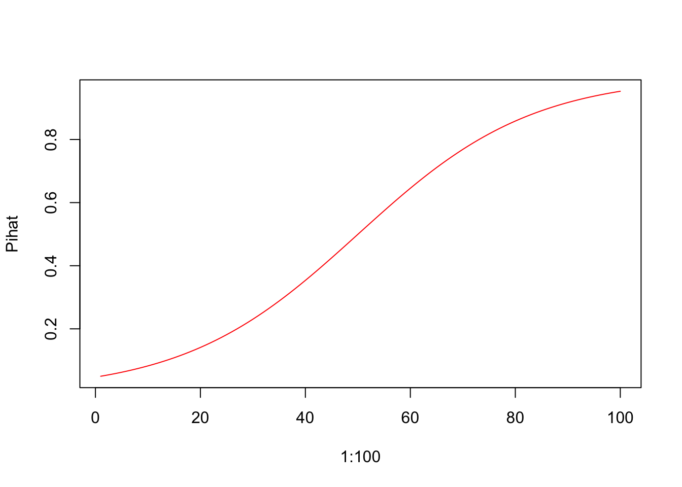
ghat=predict(model,newdata=new.data)
plot(1:100,ghat,type="l",col="red")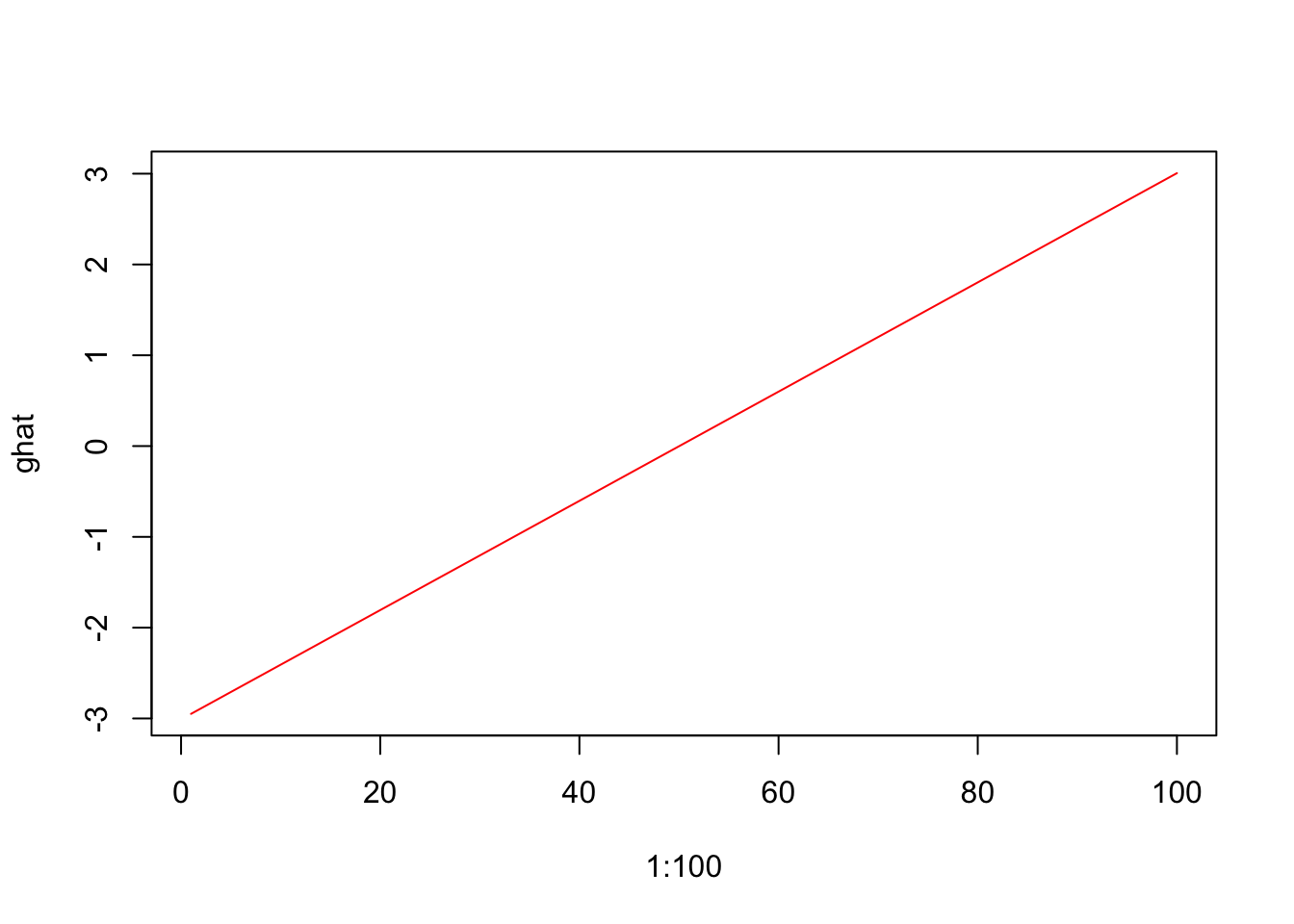

5.0.2 Plots
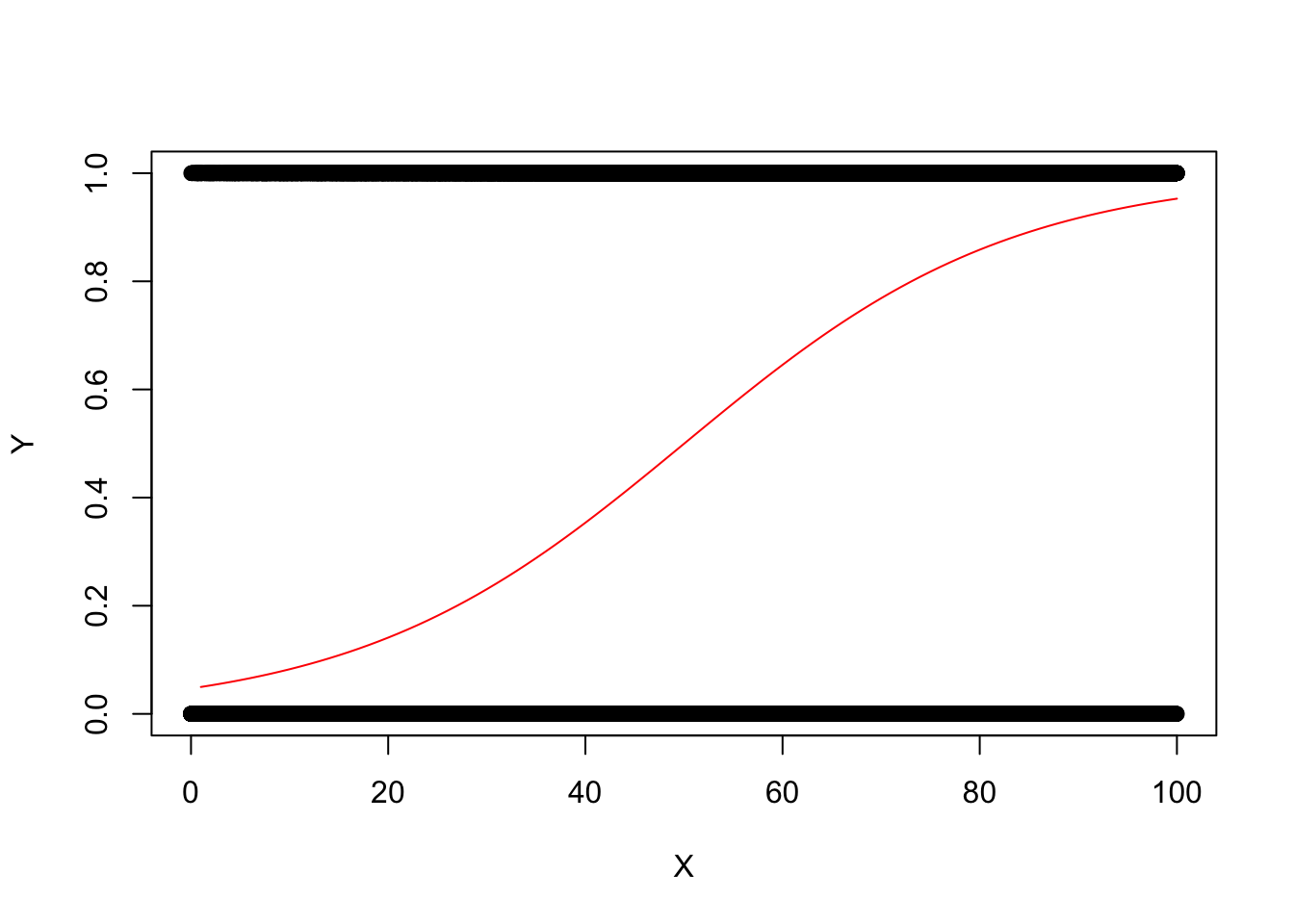
Y vs. X (Not very useful)
#Grouplot of Pihat vs X
source("http://faculty.tarleton.edu/crawford/documents/math505/LogisticRegressionFunctions.txt")

groupplot.results=groupplot(X,Y,20)
plot(groupplot.results$x,groupplot.results$Pi,
     xlab="X",
     ylab="Pihat")

lines(1:100,Pihat,col="red")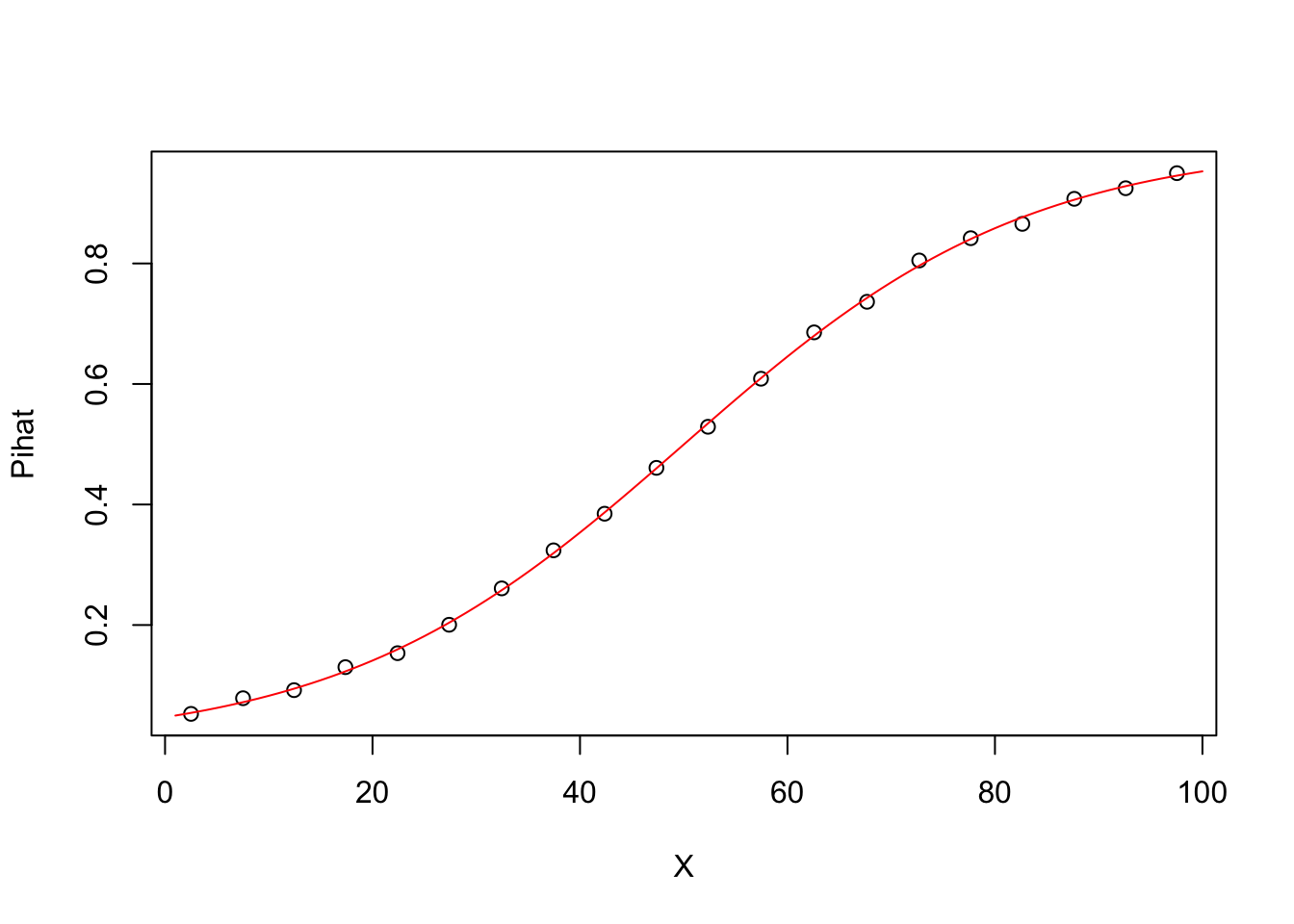
Comments The data set has been broken into 20 groups based on values of X
For each point in the plot, the x-coordinate is the average value of X in that group.
For each point in the plot, the y-coordinate is the proportion of observations in that group where Y=1. In other words, the y-coordinates provide an estimate of Pi = P(Y=1) for each group.
5.0.3 Plot of ghat vs X
group.Pihat=groupplot.results$Pi
group.ghat=log(group.Pihat/(1-group.Pihat))

plot(groupplot.results$x,group.ghat)
lines(1:100,ghat,col="red")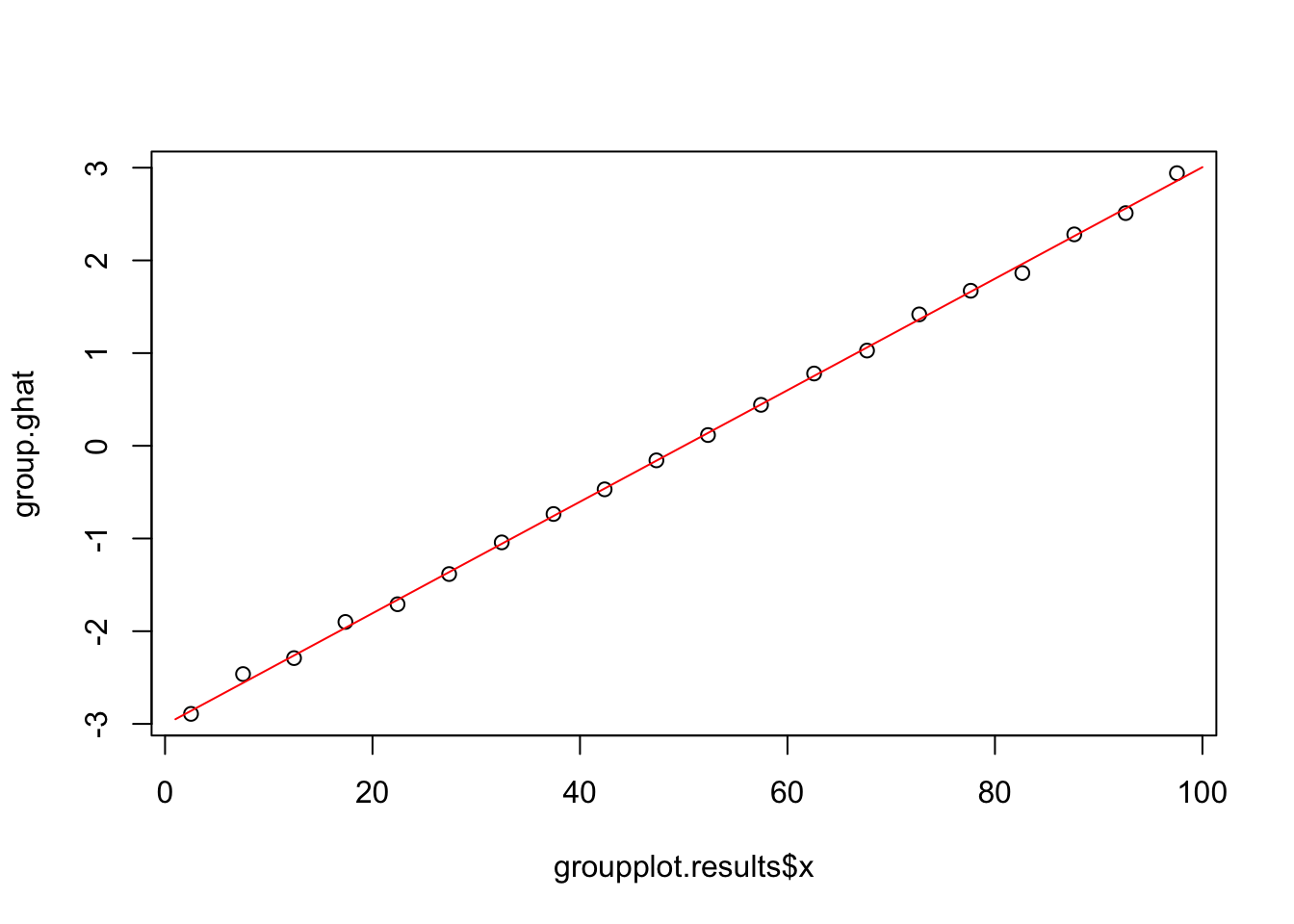
5.0.4 An Example Involving Curvature
set.seed(5366)
X=runif(100000,0,100)
g=-3+.05524*X -.002333*X^2 + .00002381*X^3
Pi=(1/(1+exp(-g)))
U=runif(100000)
Y=(U<Pi) * 1


#Degree 1 model Pihat vs X
model1=glm(Y~X,family=binomial)
summary(model1)
##
## Call:
## glm(formula = Y ~ X, family = binomial)
##
## Deviance Residuals:
## Min 1Q Median 3Q Max
## -1.3886 -0.5858 -0.2904 -0.1404 3.1861
##
## Coefficients:
## Estimate Std. Error z value Pr(>|z|)
## (Intercept) -5.0709619 0.0355466 -142.7 <2e-16 ***
## X 0.0555489 0.0004697 118.3 <2e-16 ***
## ---
## Signif. codes: 0 '***' 0.001 '**' 0.01 '*' 0.05 '.' 0.1 ' ' 1
##
## (Dispersion parameter for binomial family taken to be 1)
##
## Null deviance: 92006 on 99999 degrees of freedom
## Residual deviance: 69547 on 99998 degrees of freedom
## AIC: 69551
##
## Number of Fisher Scoring iterations: 6groupplot.results=groupplot(X,Y,20)
plot(groupplot.results$x,groupplot.results$Pi,
xlab="X",
ylab="Pihat")
x.plot.vector=1:100
Pi.plot.vector=predict(model1,
newdata=data.frame(X=x.plot.vector),
type="response")
lines(x.plot.vector,
Pi.plot.vector,
col="red")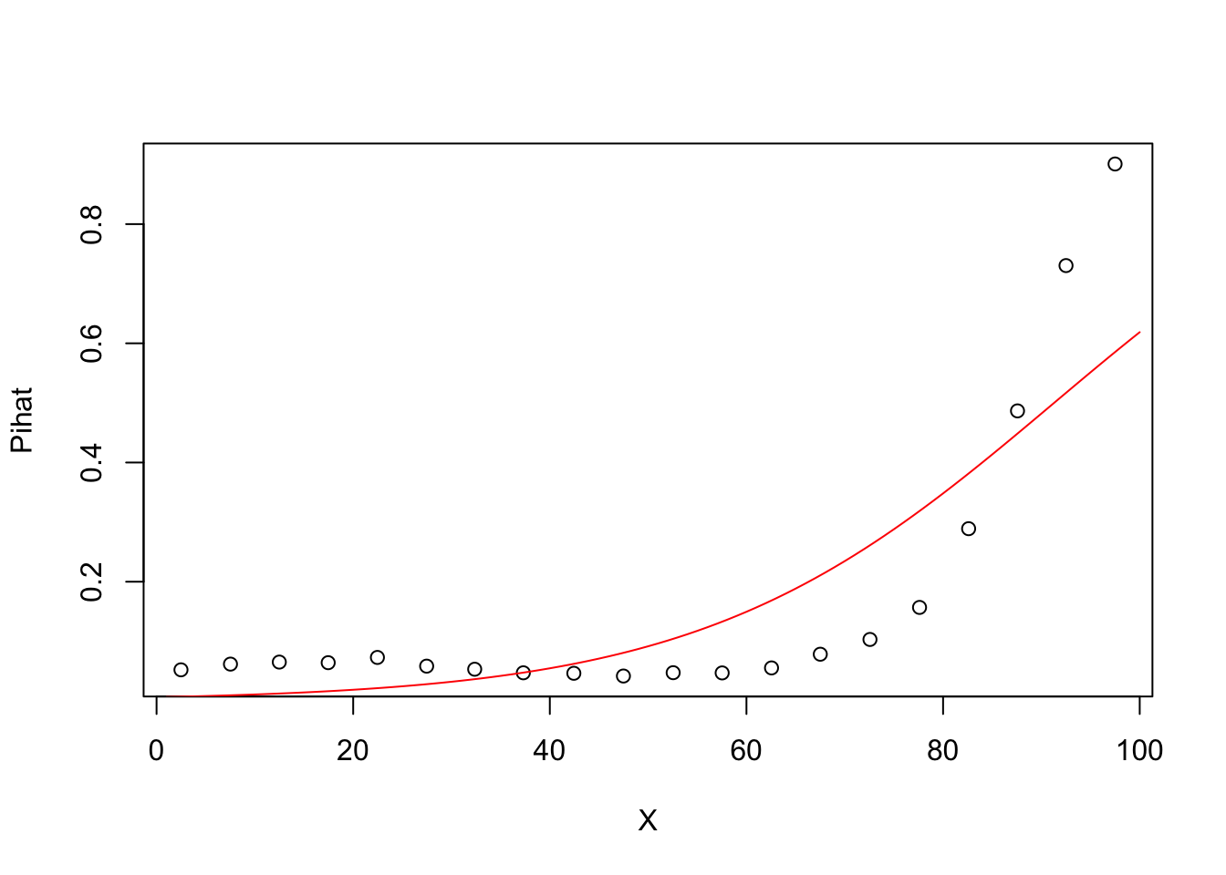
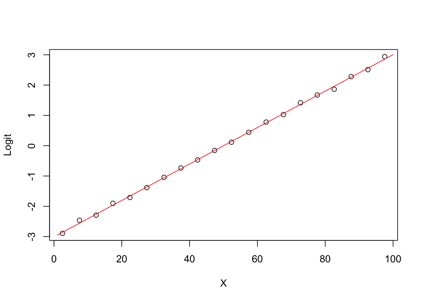
5.0.5 Degree 1 model Logit (ghat) vs X
plot(groupplot.results$x,groupplot.results$g,
     xlab="X",
     ylab="Logit")
x.plot.vector=1:100
g.plot.vector=predict(model1,
                      newdata=data.frame(X=x.plot.vector))
lines(x.plot.vector,
      g.plot.vector,
      col="red")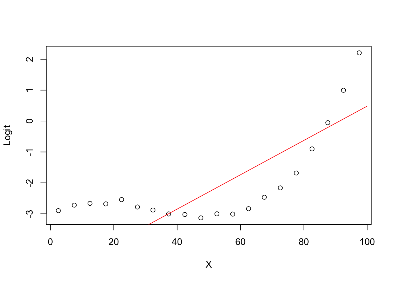
5.0.6 Degree 2 model Pihat vs X
##
## Call:
## glm(formula = Y ~ X + I(X^2), family = binomial)
##
## Deviance Residuals:
##     Min       1Q   Median       3Q      Max
## -2.0622  -0.4332  -0.2843  -0.2347   2.6938
##
## Coefficients:
##               Estimate Std. Error z value Pr(>|z|)
## (Intercept) -1.797e+00  3.373e-02  -53.27   <2e-16 ***
## X           -9.966e-02  1.568e-03  -63.56   <2e-16 ***
## I(X^2)       1.376e-03  1.501e-05   91.67   <2e-16 ***
## ---
## Signif. codes:  0 '***' 0.001 '**' 0.01 '*' 0.05 '.' 0.1 ' ' 1
##
## (Dispersion parameter for binomial family taken to be 1)
##
##     Null deviance: 92006  on 99999  degrees of freedom
## Residual deviance: 60972  on 99997  degrees of freedom
## AIC: 60978
##
## Number of Fisher Scoring iterations: 5groupplot.results=groupplot(X,Y,20)
plot(groupplot.results$x,groupplot.results$Pi,
xlab="X",
ylab="Pihat")
x.plot.vector=1:100
Pi.plot.vector=predict(model2,
newdata=data.frame(X=x.plot.vector),
type="response")
lines(x.plot.vector,
Pi.plot.vector,
col="red")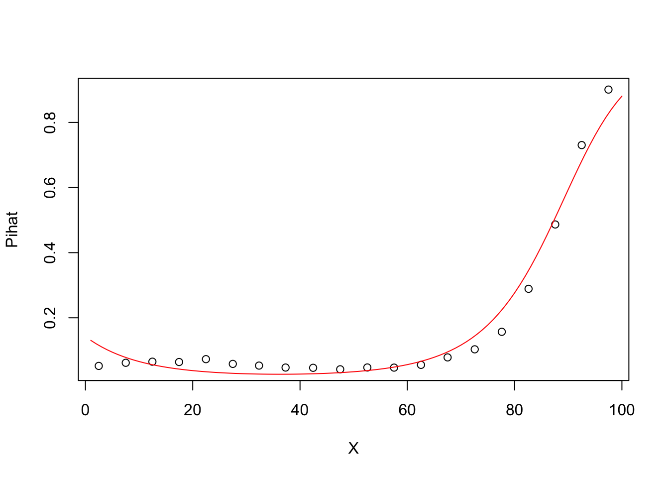
5.0.7 Degree 2 model Logit (ghat) vs X
plot(groupplot.results$x,groupplot.results$g,
     xlab="X",
     ylab="Logit")
x.plot.vector=1:100
g.plot.vector=predict(model2,
                      newdata=data.frame(X=x.plot.vector))
lines(x.plot.vector,
      g.plot.vector,
      col="red")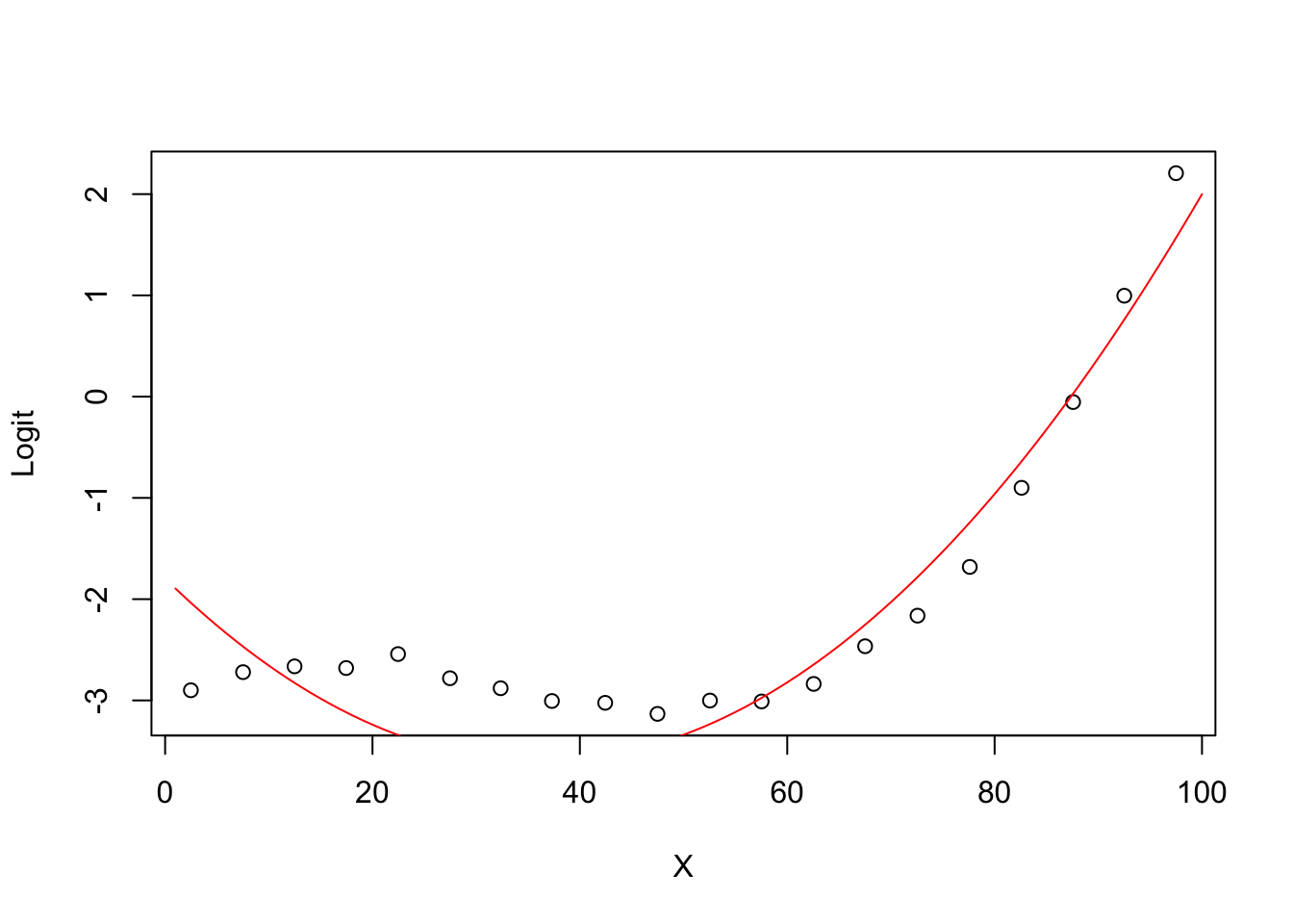
5.0.8 Degree 3 model Pihat vs X
##
## Call:
## glm(formula = Y ~ X + I(X^2) + I(X^3), family = binomial)
##
## Deviance Residuals:
##     Min       1Q   Median       3Q      Max
## -2.4714  -0.3712  -0.3361  -0.3006   2.5057
##
## Coefficients:
##               Estimate Std. Error z value Pr(>|z|)
## (Intercept) -3.026e+00  5.438e-02  -55.65   <2e-16 ***
## X            5.595e-02  4.523e-03   12.37   <2e-16 ***
## I(X^2)      -2.336e-03  9.953e-05  -23.48   <2e-16 ***
## I(X^3)       2.380e-05  6.321e-07   37.65   <2e-16 ***
## ---
## Signif. codes:  0 '***' 0.001 '**' 0.01 '*' 0.05 '.' 0.1 ' ' 1
##
## (Dispersion parameter for binomial family taken to be 1)
##
##     Null deviance: 92006  on 99999  degrees of freedom
## Residual deviance: 59457  on 99996  degrees of freedom
## AIC: 59465
##
## Number of Fisher Scoring iterations: 5groupplot.results=groupplot(X,Y,20)
plot(groupplot.results$x,groupplot.results$Pi,
xlab="X",
ylab="Pihat")
x.plot.vector=1:100
Pi.plot.vector=predict(model3,
newdata=data.frame(X=x.plot.vector),
type="response")
lines(x.plot.vector,
Pi.plot.vector,
col="red")
5.0.9 Degree 3 model Logit (ghat) vs X
plot(groupplot.results$x,groupplot.results$g,
     xlab="X",
     ylab="Logit")
x.plot.vector=1:100
g.plot.vector=predict(model3,
                      newdata=data.frame(X=x.plot.vector))
lines(x.plot.vector,
      g.plot.vector,
      col="red")
5.0.10 Degree 4 model Pihat vs X
##
## Call:
## glm(formula = Y ~ X + I(X^2) + I(X^3) + I(X^4), family = binomial)
##
## Deviance Residuals:
##     Min       1Q   Median       3Q      Max
## -2.4759  -0.3704  -0.3365  -0.3013   2.5035
##
## Coefficients:
##               Estimate Std. Error z value Pr(>|z|)
## (Intercept) -3.012e+00  6.906e-02 -43.615  < 2e-16 ***
## X            5.330e-02  9.144e-03   5.829 5.58e-09 ***
## I(X^2)      -2.221e-03  3.595e-04  -6.179 6.44e-10 ***
## I(X^3)       2.207e-05  5.239e-06   4.212 2.53e-05 ***
## I(X^4)       8.449e-09  2.534e-08   0.333    0.739
## ---
## Signif. codes:  0 '***' 0.001 '**' 0.01 '*' 0.05 '.' 0.1 ' ' 1
##
## (Dispersion parameter for binomial family taken to be 1)
##
##     Null deviance: 92006  on 99999  degrees of freedom
## Residual deviance: 59457  on 99995  degrees of freedom
## AIC: 59467
##
## Number of Fisher Scoring iterations: 5groupplot.results=groupplot(X,Y,20)
plot(groupplot.results$x,groupplot.results$Pi,
xlab="X",
ylab="Pihat")
x.plot.vector=1:100
Pi.plot.vector=predict(model4,
newdata=data.frame(X=x.plot.vector),
type="response")
lines(x.plot.vector,
Pi.plot.vector,
col="red")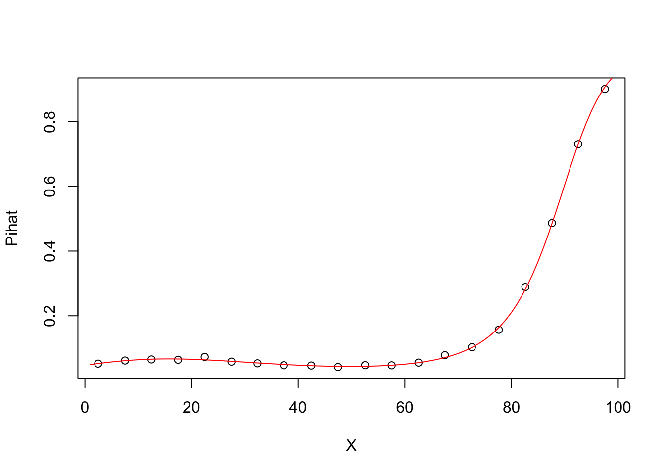
5.0.11 Degree 4 model Logit (ghat) vs X
plot(groupplot.results$x,groupplot.results$g,
     xlab="X",
     ylab="Logit")
x.plot.vector=1:100
g.plot.vector=predict(model4,
                      newdata=data.frame(X=x.plot.vector))
lines(x.plot.vector,
      g.plot.vector,
      col="red")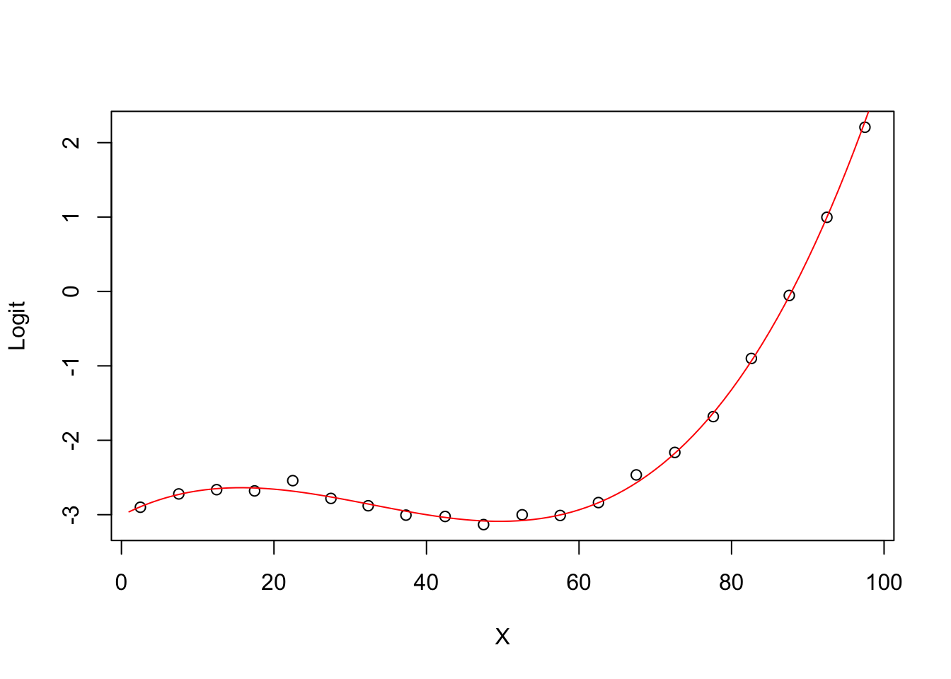
5.1 Testing model1 vs model3
G=model1$deviance-model3$deviance
pchisq(G,lower.tail=FALSE,df=model1$df.residual-model2$df.residual)
## [1] 0## [1] 0## [1] 0.73880445.2 A Multivariate Example
set.seed(5366)
Rank=rnorm(200,.67,.1)
SAT=round(rnorm(200,980,132),-1)
ShoeSize=round(rnorm(200,9,1),1)
U=runif(200,0,1)
Mother=1:200


for(i in 1:200){
  if(U[i]<.5){Mother[i]="SomeCollege"}
  if((U[i]>.5)&(U[i]<.8)){Mother[i]="Bachelors"}
  if((U[i]>.8)&(U[i]<.95)){Mother[i]="HighSchool"}
  if(U[i]>0.95){Mother[i]="GradDegree"}
}


Mother=as.factor(Mother)
Mother=relevel(Mother,4)


tempmodel=lm(1:200~Rank+SAT+Mother)
X=model.matrix(tempmodel)
beta=c(-9.3,10,.00364,1.5,1.5,0)
g=X%*%beta
Pi=1/(1+exp(-g))
U2=runif(200,0,1)
Retention=(U2<Pi)*1
Retention.data=data.frame(Rank,SAT,ShoeSize,Mother)

#Fitting a model
model=glm(Retention~.,data=Retention.data,family=binomial)
summary(model)
##
## Call:
## glm(formula = Retention ~ ., family = binomial, data = Retention.data)
##
## Deviance Residuals:
## Min 1Q Median 3Q Max
## -2.7118 0.1951 0.3948 0.6374 1.3498
##
## Coefficients:
## Estimate Std. Error z value Pr(>|z|)
## (Intercept) -8.293975 3.095703 -2.679 0.007380 **
## Rank 10.277291 2.467877 4.164 3.12e-05 ***
## SAT 0.004871 0.001576 3.090 0.002002 **
## ShoeSize -0.233967 0.207032 -1.130 0.258435
## MotherBachelors 1.927406 0.555780 3.468 0.000524 ***
## MotherGradDegree 0.882259 1.180404 0.747 0.454809
## MotherHighSchool -0.028233 0.514632 -0.055 0.956249
## ---
## Signif. codes: 0 '***' 0.001 '**' 0.01 '*' 0.05 '.' 0.1 ' ' 1
##
## (Dispersion parameter for binomial family taken to be 1)
##
## Null deviance: 197.36 on 199 degrees of freedom
## Residual deviance: 156.62 on 193 degrees of freedom
## AIC: 170.62
##
## Number of Fisher Scoring iterations: 5Better Plotting Function
quantlogitplot=function(Y,x,degree,xname,Yname,numgroups,yrange){
  xrange=range(x)
  n=length(Y)
  X=rep(1,n)
  for(i in 1:degree){
    X=cbind(X,x^i)
  }
  model=glm(Y~X-1,family='binomial')
  L=groupplot(x,Y,numgroups)
  plot(L$x,L$g,xlab=xname,ylab=Yname,ylim=yrange)
  a=xrange[1]
  b=xrange[2]
  index=(1:100)/100
  index=a+(b-a)*index
  Index=rep(1,100)
  for(i in 1:degree){
    Index=cbind(Index,index^i)
  }
  betahat=coef(model)
  lines(index,Index%*%betahat,col='red')


}
Rank model
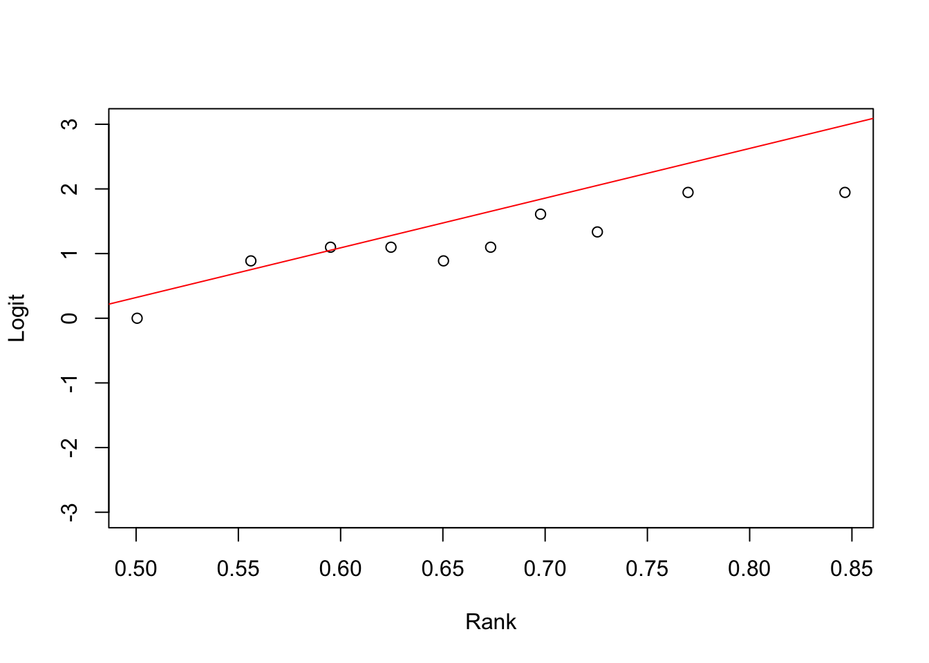
rank.model=glm(Retention~Rank,family=binomial)
rank.model.2=glm(Retention~Rank+I(Rank^2),family=binomial)
summary(rank.model)
##
## Call:
## glm(formula = Retention ~ Rank, family = binomial)
##
## Deviance Residuals:
## Min 1Q Median 3Q Max
## -2.6285 0.3307 0.5337 0.7007 1.1764
##
## Coefficients:
## Estimate Std. Error z value Pr(>|z|)
## (Intercept) -3.522 1.339 -2.631 0.008505 **
## Rank 7.685 2.124 3.619 0.000296 ***
## ---
## Signif. codes: 0 '***' 0.001 '**' 0.01 '*' 0.05 '.' 0.1 ' ' 1
##
## (Dispersion parameter for binomial family taken to be 1)
##
## Null deviance: 197.36 on 199 degrees of freedom
## Residual deviance: 182.27 on 198 degrees of freedom
## AIC: 186.27
##
## Number of Fisher Scoring iterations: 5##
## Call:
## glm(formula = Retention ~ Rank + I(Rank^2), family = binomial)
##
## Deviance Residuals:
## Min 1Q Median 3Q Max
## -2.4764 0.3629 0.5269 0.6848 1.2464
##
## Coefficients:
## Estimate Std. Error z value Pr(>|z|)
## (Intercept) -6.161 7.049 -0.874 0.382
## Rank 16.100 22.111 0.728 0.467
## I(Rank^2) -6.574 17.137 -0.384 0.701
##
## (Dispersion parameter for binomial family taken to be 1)
##
## Null deviance: 197.36 on 199 degrees of freedom
## Residual deviance: 182.12 on 197 degrees of freedom
## AIC: 188.12
##
## Number of Fisher Scoring iterations: 5## [1] 0.7062637SAT model

SAT.model=glm(Retention~SAT,family=binomial)
SAT.model.2=glm(Retention~SAT+I(SAT^2),family=binomial)
summary(SAT.model)
##
## Call:
## glm(formula = Retention ~ SAT, family = binomial)
##
## Deviance Residuals:
## Min 1Q Median 3Q Max
## -2.1306 0.4343 0.5911 0.7097 1.0585
##
## Coefficients:
## Estimate Std. Error z value Pr(>|z|)
## (Intercept) -2.020442 1.342033 -1.506 0.1322
## SAT 0.003604 0.001422 2.534 0.0113 *
## ---
## Signif. codes: 0 '***' 0.001 '**' 0.01 '*' 0.05 '.' 0.1 ' ' 1
##
## (Dispersion parameter for binomial family taken to be 1)
##
## Null deviance: 197.36 on 199 degrees of freedom
## Residual deviance: 190.36 on 198 degrees of freedom
## AIC: 194.36
##
## Number of Fisher Scoring iterations: 4##
## Call:
## glm(formula = Retention ~ SAT + I(SAT^2), family = binomial)
##
## Deviance Residuals:
## Min 1Q Median 3Q Max
## -2.1492 0.4182 0.5974 0.7177 0.9973
##
## Coefficients:
## Estimate Std. Error z value Pr(>|z|)
## (Intercept) -3.841e-01 7.425e+00 -0.052 0.959
## SAT 1.239e-04 1.561e-02 0.008 0.994
## I(SAT^2) 1.817e-06 8.128e-06 0.224 0.823
##
## (Dispersion parameter for binomial family taken to be 1)
##
## Null deviance: 197.36 on 199 degrees of freedom
## Residual deviance: 190.31 on 197 degrees of freedom
## AIC: 196.31
##
## Number of Fisher Scoring iterations: 5## [1] 0.821137Shoe Size model
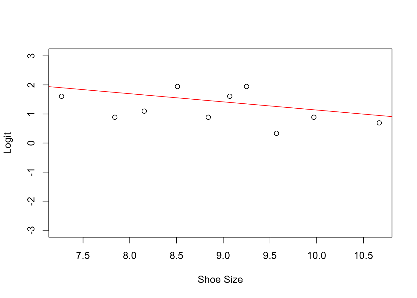
##
## Call:
## glm(formula = Retention ~ ShoeSize, family = binomial)
##
## Deviance Residuals:
##     Min       1Q   Median       3Q      Max
## -2.0653   0.5434   0.6263   0.6758   0.8619
##
## Coefficients:
##             Estimate Std. Error z value Pr(>|z|)
## (Intercept)   3.9444     1.6823   2.345    0.019 *
## ShoeSize     -0.2808     0.1843  -1.524    0.128
## ---
## Signif. codes:  0 '***' 0.001 '**' 0.01 '*' 0.05 '.' 0.1 ' ' 1
##
## (Dispersion parameter for binomial family taken to be 1)
##
##     Null deviance: 197.36  on 199  degrees of freedom
## Residual deviance: 195.00  on 198  degrees of freedom
## AIC: 199
##
## Number of Fisher Scoring iterations: 4
Mother’s Education Level
## Mother
## SomeCollege   Bachelors  GradDegree  HighSchool
## 89 71 6 34##
## Call:
## glm(formula = Retention ~ ., family = binomial, data = Retention.data)
##
## Deviance Residuals:
## Min 1Q Median 3Q Max
## -2.7118 0.1951 0.3948 0.6374 1.3498
##
## Coefficients:
## Estimate Std. Error z value Pr(>|z|)
## (Intercept) -8.293975 3.095703 -2.679 0.007380 **
## Rank 10.277291 2.467877 4.164 3.12e-05 ***
## SAT 0.004871 0.001576 3.090 0.002002 **
## ShoeSize -0.233967 0.207032 -1.130 0.258435
## MotherBachelors 1.927406 0.555780 3.468 0.000524 ***
## MotherGradDegree 0.882259 1.180404 0.747 0.454809
## MotherHighSchool -0.028233 0.514632 -0.055 0.956249
## ---
## Signif. codes: 0 '***' 0.001 '**' 0.01 '*' 0.05 '.' 0.1 ' ' 1
##
## (Dispersion parameter for binomial family taken to be 1)
##
## Null deviance: 197.36 on 199 degrees of freedom
## Residual deviance: 156.62 on 193 degrees of freedom
## AIC: 170.62
##
## Number of Fisher Scoring iterations: 5##
## Call:
## glm(formula = Retention ~ Rank + SAT + ShoeSize, family = binomial,
## data = Retention.data)
##
## Deviance Residuals:
## Min 1Q Median 3Q Max
## -2.3186 0.2787 0.4652 0.6840 1.3253
##
## Coefficients:
## Estimate Std. Error z value Pr(>|z|)
## (Intercept) -5.576068 2.787273 -2.001 0.045441 *
## Rank 7.552550 2.170519 3.480 0.000502 ***
## SAT 0.003959 0.001482 2.670 0.007580 **
## ShoeSize -0.182597 0.195038 -0.936 0.349163
## ---
## Signif. codes: 0 '***' 0.001 '**' 0.01 '*' 0.05 '.' 0.1 ' ' 1
##
## (Dispersion parameter for binomial family taken to be 1)
##
## Null deviance: 197.36 on 199 degrees of freedom
## Residual deviance: 173.74 on 196 degrees of freedom
## AIC: 181.74
##
## Number of Fisher Scoring iterations: 5## [1] 0.0006693412Recoding Mother’s Education Level
## Mother
## SomeCollege   Bachelors  GradDegree  HighSchool
## 89 71 6 34##
## 1 2 3 4
## 89 71 6 34Mother.Recode=c("HighSchool/SomeCollege",
"Bachelors/GradDegree",
"Bachelors/GradDegree",
"HighSchool/SomeCollege"
)
Mother2=Mother.Recode[Mother]
table(Mother2)## Mother2
## Bachelors/GradDegree HighSchool/SomeCollege
## 77 123##
## Call:
## glm(formula = Retention ~ Rank + SAT + ShoeSize + Mother2, family = binomial,
## data = Retention.data)
##
## Deviance Residuals:
## Min 1Q Median 3Q Max
## -2.6724 0.2069 0.4023 0.6406 1.3438
##
## Coefficients:
## Estimate Std. Error z value Pr(>|z|)
## (Intercept) -6.339209 2.964094 -2.139 0.03246 *
## Rank 10.073942 2.417513 4.167 3.09e-05 ***
## SAT 0.004881 0.001572 3.104 0.00191 **
## ShoeSize -0.235572 0.206512 -1.141 0.25399
## Mother2HighSchool/SomeCollege -1.827392 0.500327 -3.652 0.00026 ***
## ---
## Signif. codes: 0 '***' 0.001 '**' 0.01 '*' 0.05 '.' 0.1 ' ' 1
##
## (Dispersion parameter for binomial family taken to be 1)
##
## Null deviance: 197.36 on 199 degrees of freedom
## Residual deviance: 157.24 on 195 degrees of freedom
## AIC: 167.24
##
## Number of Fisher Scoring iterations: 5## [1] 0.7323225Removing Shoe Size
##
## Call:
## glm(formula = Retention ~ Rank + SAT + Mother2, family = binomial,
##     data = Retention.data)
##
## Deviance Residuals:
##     Min       1Q   Median       3Q      Max
## -2.6402   0.2009   0.4144   0.6228   1.3829
##
## Coefficients:
##                                Estimate Std. Error z value Pr(>|z|)
## (Intercept)                   -8.683127   2.187868  -3.969 7.22e-05 ***
## Rank                          10.436952   2.409344   4.332 1.48e-05 ***
## SAT                            0.004852   0.001561   3.107 0.001887 **
## Mother2HighSchool/SomeCollege -1.793748   0.496847  -3.610 0.000306 ***
## ---
## Signif. codes:  0 '***' 0.001 '**' 0.01 '*' 0.05 '.' 0.1 ' ' 1
##
## (Dispersion parameter for binomial family taken to be 1)
##
##     Null deviance: 197.36  on 199  degrees of freedom
## Residual deviance: 158.57  on 196  degrees of freedom
## AIC: 166.57
##
## Number of Fisher Scoring iterations: 5## [1] 0.5841335.2.1 Variable Selection
Stepwise
## Start:  AIC=170.62
## Retention ~ Rank + SAT + ShoeSize + Mother
##
##            Df Deviance    AIC
## - ShoeSize  1   157.92 169.92
## <none>          156.62 170.62
## - SAT       1   167.33 179.33
## - Mother    3   173.74 181.74
## - Rank      1   178.21 190.21
##
## Step:  AIC=169.92
## Retention ~ Rank + SAT + Mother
##
##          Df Deviance    AIC
## <none>        157.92 169.92
## - SAT     1   168.57 178.57
## - Mother  3   174.62 180.62
## - Rank    1   181.53 191.53
#Best Subsets
library(bestglm)
X=model.matrix(model)
X=X[,2:(ncol(X))]
y=Retention
Xy=data.frame(X,y)
best.model=bestglm(Xy,family=binomial)## Morgan-Tatar search since family is non-gaussian.## [1] "BestModel" "BestModels" "Bestq" "qTable" "Subsets" "Title"
## [7] "ModelReport"##
## Call:
## glm(formula = y ~ ., family = family, data = Xi, weights = weights)
##
## Deviance Residuals:
## Min 1Q Median 3Q Max
## -2.6715 0.1966 0.4066 0.6264 1.3696
##
## Coefficients:
## Estimate Std. Error z value Pr(>|z|)
## (Intercept) -10.429845 2.332693 -4.471 7.78e-06 ***
## Rank 10.610051 2.447711 4.335 1.46e-05 ***
## SAT 0.004724 0.001547 3.054 0.002257 **
## MotherBachelors 1.857860 0.518495 3.583 0.000339 ***
## ---
## Signif. codes: 0 '***' 0.001 '**' 0.01 '*' 0.05 '.' 0.1 ' ' 1
##
## (Dispersion parameter for binomial family taken to be 1)
##
## Null deviance: 197.36 on 199 degrees of freedom
## Residual deviance: 158.45 on 196 degrees of freedom
## AIC: 166.45
##
## Number of Fisher Scoring iterations: 55.3 Assessing Model Performance and Fit
source("http://faculty.tarleton.edu/crawford/documents/Math5364/MiscRFunctions.txt")

#Training Data
Retention.data.2=data.frame(Retention,Rank,SAT,Mother2)
train=trainsample(Retention.data.2,0.7)


#Fitting Model

model=glm(Retention~.,
          data=Retention.data.2[train,],
          family=binomial)
summary(model)
##
## Call:
## glm(formula = Retention ~ ., family = binomial, data = Retention.data.2[train,
## ])
##
## Deviance Residuals:
## Min 1Q Median 3Q Max
## -2.4849 0.1980 0.4345 0.6524 1.3690
##
## Coefficients:
## Estimate Std. Error z value Pr(>|z|)
## (Intercept) -9.168525 2.582276 -3.551 0.000384 ***
## Rank 10.491690 2.887293 3.634 0.000279 ***
## SAT 0.005166 0.001989 2.597 0.009392 **
## Mother2HighSchool/SomeCollege -1.734604 0.581591 -2.983 0.002859 **
## ---
## Signif. codes: 0 '***' 0.001 '**' 0.01 '*' 0.05 '.' 0.1 ' ' 1
##
## (Dispersion parameter for binomial family taken to be 1)
##
## Null deviance: 142.84 on 139 degrees of freedom
## Residual deviance: 115.67 on 136 degrees of freedom
## AIC: 123.67
##
## Number of Fisher Scoring iterations: 5Classification Accuracy
#confmatrix function from previous tutorial
confmatrix=function(y,predy){
  matrix=table(y,predy)
  accuracy=sum(diag(matrix))/sum(matrix)
  return(list(matrix=matrix,accuracy=accuracy,error=1-accuracy))
}

Pihat=predict(model,
              newdata=Retention.data.2[-train,],
              type="response")
pred.retention=(Pihat>=0.5)*1
table(pred.retention)
## pred.retention
## 0 1
## 8 52## $matrix
## predy
## y 0 1
## 0 5 5
## 1 3 47
##
## $accuracy
## [1] 0.8666667
##
## $error
## [1] 0.1333333ROC Curve
## Setting levels: control = 0, case = 1## Setting direction: controls < cases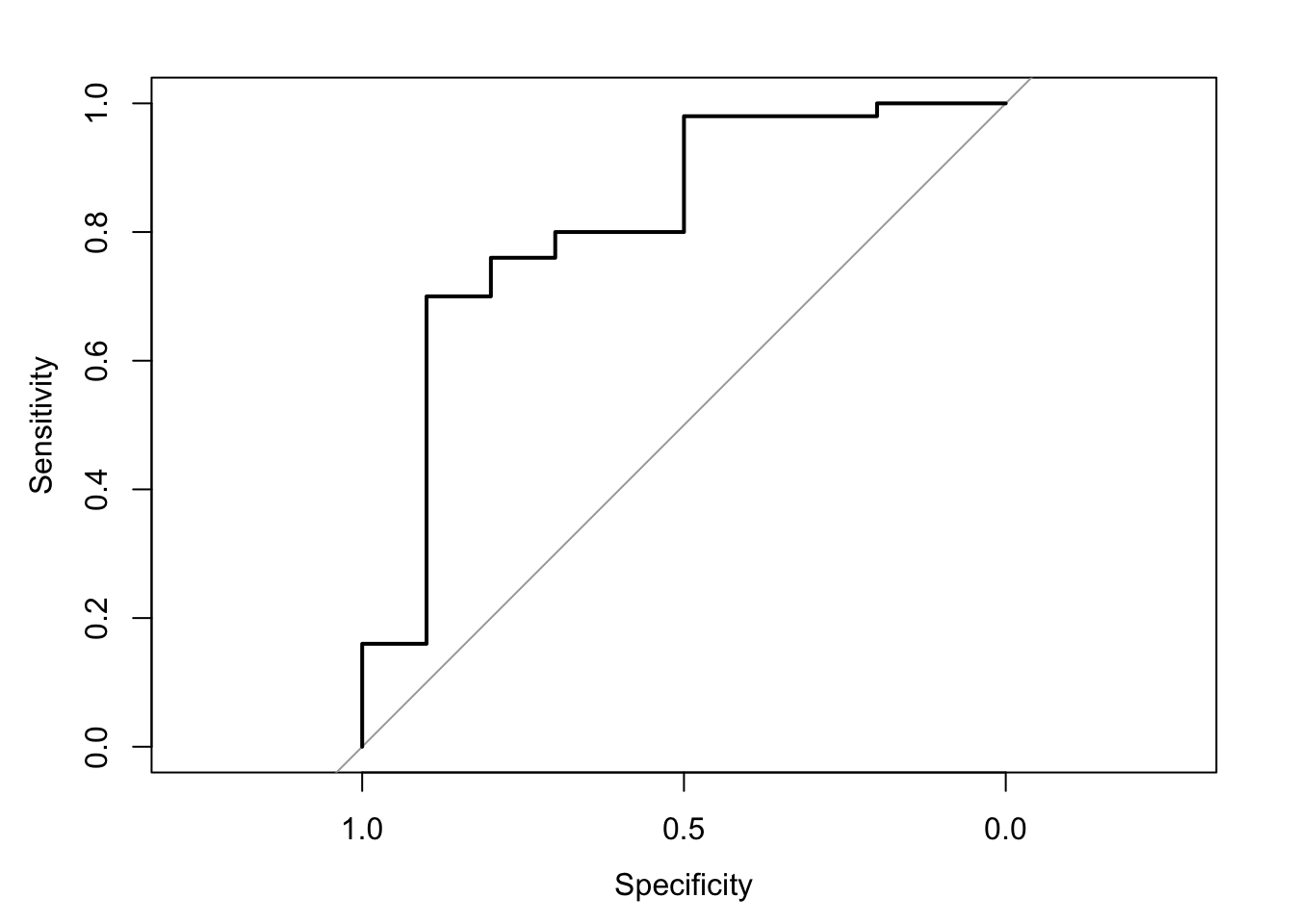
Hosmer-Lemeshow Goodness-of-fit Test
# dependecy doesnt exist cant use
# Hosmer-Lemeshow goodness of fit tests from this package
# library(MKmisc)

model=glm(Retention~.,
          data=Retention.data.2,
          family=binomial)

Pihat=predict(model,
              type="response")

# HLgof.test(fit=Pihat,obs=Retention)
Visualizing HLgof.test
hlgof=function(pihat,Y,ngr){
  sortframe=sort(pihat,index=TRUE)
  pihat=sortframe$x
  Y=Y[sortframe$ix]
  s=floor(length(pihat)/ngr)  #groupsize
  pipred=1:ngr
  piobs=1:ngr
  Chat=0

  for(i in 1:ngr){
    index=(((i-1)*s+1):(i*s))
    if(i==ngr){index=(((i-1)*s+1):(length(pihat)))}
    pipred[i]=mean(pihat[index])
    nk=length(index)
    ok=sum(Y[index])
    piobs[i]=ok/nk
    Chat=Chat+(ok-nk*pipred[i])^2/(nk*pipred[i]*(1-pipred[i]))}

  pvalue=1-pchisq(Chat,ngr-2)
  return(list(pipred=pipred,piobs=piobs,Chat=Chat,pvalue=pvalue))}


hlgof.results=hlgof(Pihat,Retention,10)
Comparing Pihat and Piobs
plot(hlgof.results$pipred,hlgof.results$piobs,
     xlim=c(0,1),
     ylim=c(0,1))
lines((1:100)/100,(1:100)/100,col="red")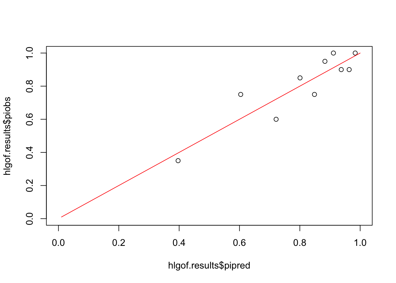
##       piobs    pipred
##  [1,]  0.35 0.3965338
##  [2,]  0.75 0.6039958
##  [3,]  0.60 0.7213944
##  [4,]  0.85 0.8006625
##  [5,]  0.75 0.8485368
##  [6,]  0.95 0.8831521
##  [7,]  1.00 0.9113384
##  [8,]  0.90 0.9372917
##  [9,]  0.90 0.9635551
## [10,] 1.00 0.9835395## piobs pipred
## [1,] 7 7.930676
## [2,] 15 12.079916
## [3,] 12 14.427888
## [4,] 17 16.013249
## [5,] 15 16.970736
## [6,] 19 17.663041
## [7,] 20 18.226769
## [8,] 18 18.745833
## [9,] 18 19.271102
## [10,] 20 19.670789## [1] 11.1661