Chapter 10 Clustering Techniques
10.0.1 k-means
Generating some data
set.seed(5364)
x1=rnorm(100,5,1)
x2=rnorm(100,15,1)
x3=rnorm(100,10,1)

y1=rnorm(100,10,1)
y2=rnorm(100,10,1)
y3=rnorm(100,20,1)

mydata=data.frame(x=c(x1,x2,x3),y=c(y1,y2,y3))
plot(y~x,data=mydata,asp=1)
Finding clusters with kmeans
kmeans.output=kmeans(mydata,centers=3)
clusters=kmeans.output$cluster
colvect=c("red","green","blue")
plot(y~x,data=mydata,col=colvect[clusters],asp=1)
Centers of clusters
centers=kmeans.output$centers
plot(y~x,data=mydata,col=colvect[clusters],asp=1)
points(centers,col='black',pch=24,bg='black')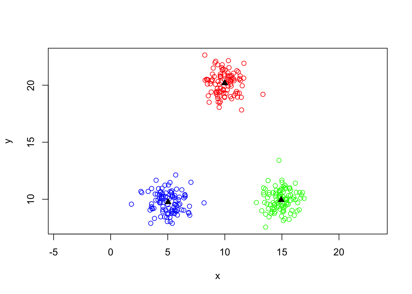
Sums of squares for kmeans
## [1] 12561.82## [1] 179.8380 164.9543 187.9353## [1] 532.7276## [1] 12029.09## [1] 12561.82Bad choice of initial centers
centers0=cbind(c(9,10,11),c(20,10,20))
kout=kmeans(mydata,centers=centers0)
plot(y~x,data=mydata,col=colvect[kout$cluster],asp=1)
points(centers0,col='black',pch=24,bg='black')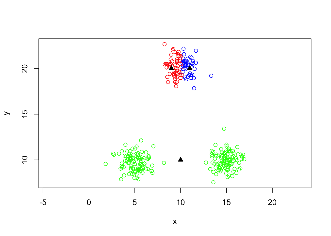
## [1] 5385.793Repeating k-means a large number of random times
repeat.kmeans=function(data,centers,repetitions){
  best.kmeans=NULL
  best.ssw=Inf

  for(i in 1:repetitions){
    kmeans.temp=kmeans(x=data,centers=centers)
    if(kmeans.temp$tot.withinss<best.ssw){
      best.ssw=kmeans.temp$tot.withinss
      best.kmeans=kmeans.temp
    }
  }
  return(best.kmeans)
}


best=repeat.kmeans(mydata,3,1000)
best$tot.withinss
## [1] 532.7276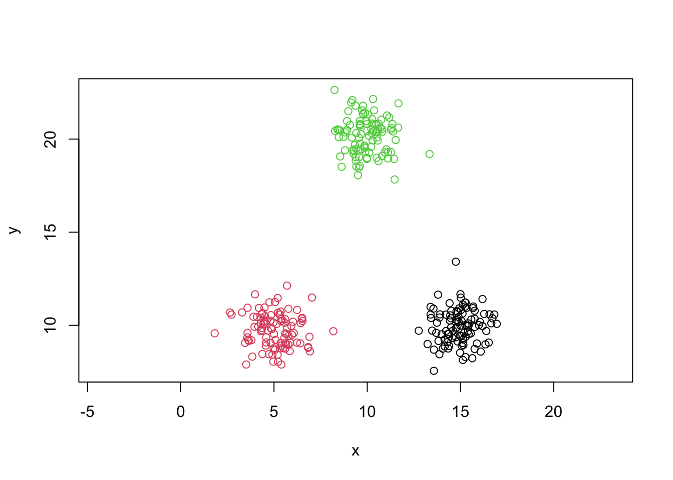
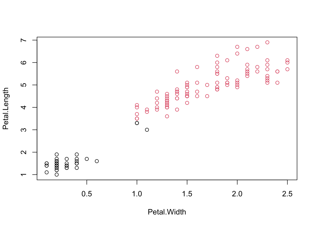
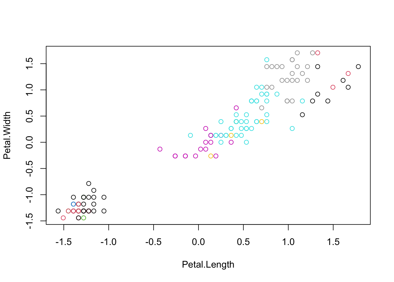
k-means for iris data
##
##     setosa versicolor virginica
##   1     50          0         0
##   2      0         48        14
##   3      0          2        36
10.0.2 CLUSTER EVALUATION
Generating data
set.seed(5364)
x1=rnorm(100,5,1)
x2=rnorm(100,15,1)
x3=rnorm(100,10,1)

y1=rnorm(100,10,1)
y2=rnorm(100,10,1)
y3=rnorm(100,20,1)

mydata=data.frame(x=c(x1,x2,x3),y=c(y1,y2,y3))
plot(y~x,data=mydata,asp=1)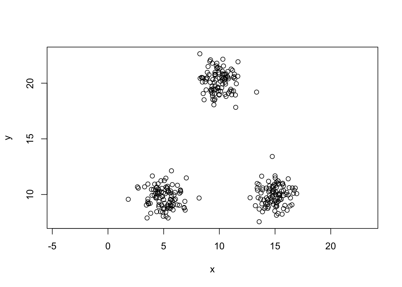
repeat.kmeans
repeat.kmeans=function(data,centers,repetitions){
  best.kmeans=NULL
  best.ssw=Inf

  for(i in 1:repetitions){
    kmeans.temp=kmeans(x=data,centers=centers)
    if(kmeans.temp$tot.withinss<best.ssw){
      best.ssw=kmeans.temp$tot.withinss
      best.kmeans=kmeans.temp
    }
  }
  return(best.kmeans)
}


#repetitions needed
min.rep=function(K,epsilon){
  ceiling(log(epsilon)/log(1-factorial(K)/K^K))
}

min.rep(3,.01)
## [1] 19## [1] 532.7276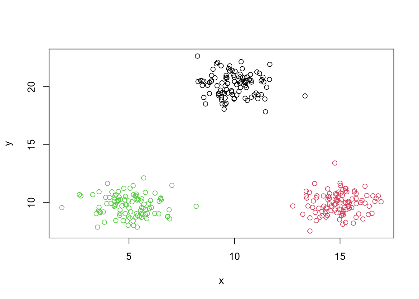
## [1] 12689## [1] 206.4282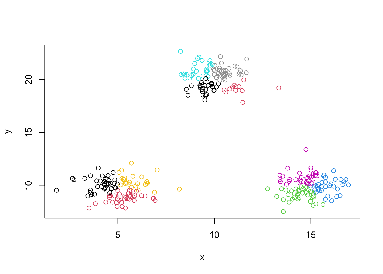
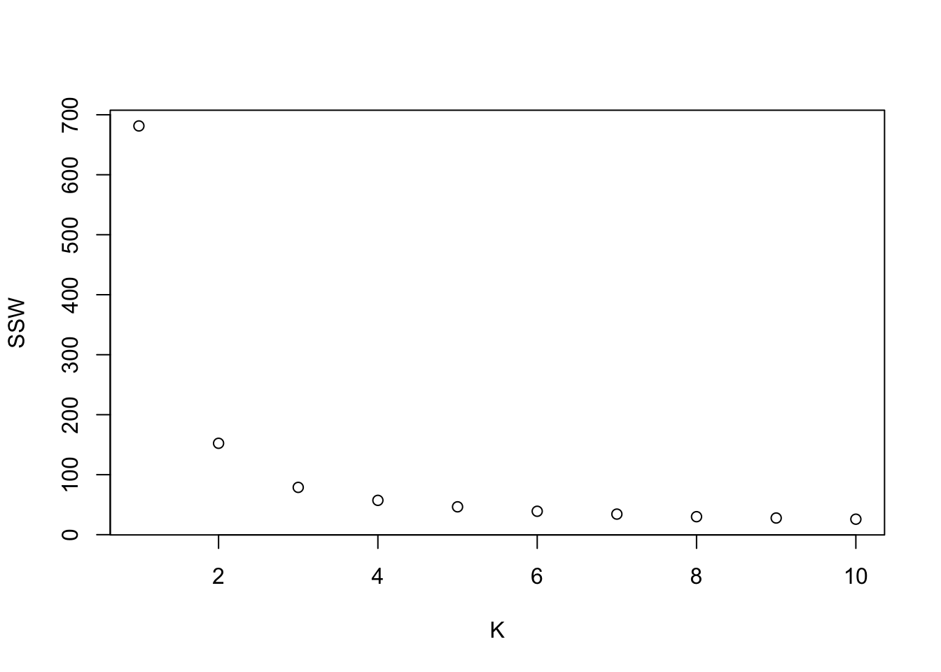
10.1 Plotting SSW vs K
plot.ssw=function(data,max.K,max.iter,epsilon){
  ssw.vect=1:max.K
  for(K in 1:max.K){
    iter=min(max.iter,min.rep(K,epsilon))
    kmeans.temp=repeat.kmeans(data,K,iter)
    ssw.vect[K]=kmeans.temp$tot.withinss
  }
  plot(1:max.K,ssw.vect,xlab="K",ylab="SSW")
}

plot.ssw(mydata,10,1000,.01)
plot.ssw(mydata,10,20000,.01)  #Same results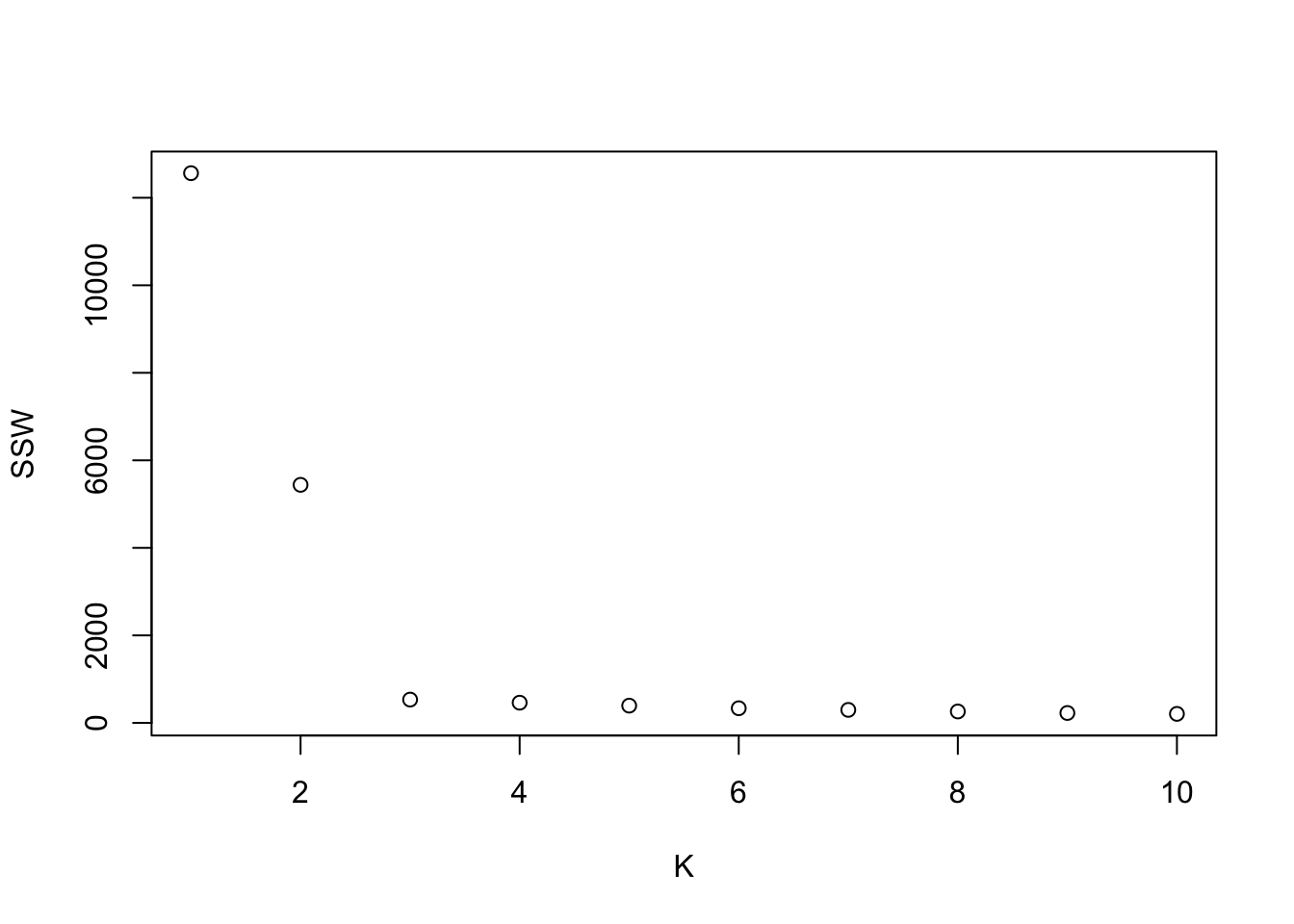
10.1.1 Silhouette coefficient
## [1] 532.7276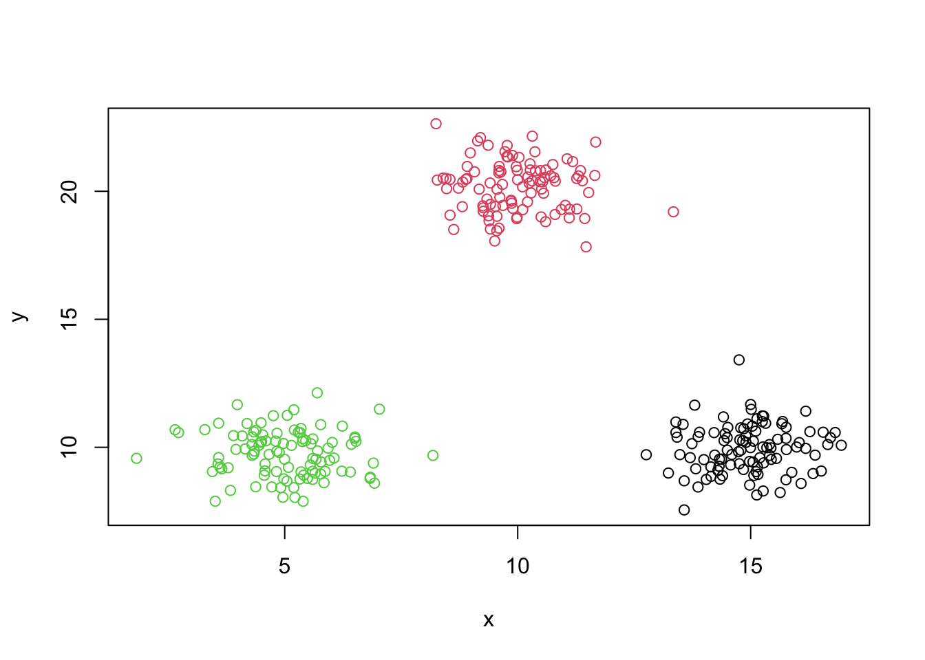
#Distance matrix
library(fields)
dmatrix=rdist(mydata)


#Inefficient distance matrix function
distance.matrix=function(data){
  n=nrow(data)
  dmatrix=matrix(nrow=n,ncol=n)
  for(i in 1:n){
    for(j in 1:n){
      dmatrix[i,j]=sum((data[i,]-data[j,])^2)
    }
  }
  return(sqrt(dmatrix))
}

dmatrix2=distance.matrix(mydata)

range(dmatrix-dmatrix2)
## [1] 0 0## cluster neighbor sil_width
## [1,] 3 1 0.8696676
## [2,] 3 2 0.8088582
## [3,] 3 1 0.8247808
## [4,] 3 1 0.8709415
## [5,] 3 1 0.7229257
## [6,] 3 1 0.8550709
## [7,] 3 1 0.8493582
## [8,] 3 1 0.8078686
## [9,] 3 1 0.8290648
## [10,] 3 1 0.8713395
## [11,] 3 1 0.8614949
## [12,] 3 1 0.8404844
## [13,] 3 1 0.8382013
## [14,] 3 1 0.8125570
## [15,] 3 1 0.8744478
## [16,] 3 1 0.8477436
## [17,] 3 1 0.8771452
## [18,] 3 1 0.7719118
## [19,] 3 1 0.8699126
## [20,] 3 1 0.8595228
## [21,] 3 1 0.8468149
## [22,] 3 1 0.8709906
## [23,] 3 2 0.8074481
## [24,] 3 1 0.8608883
## [25,] 3 1 0.8354594
## [26,] 3 2 0.7800963
## [27,] 3 1 0.8085929
## [28,] 3 1 0.8337341
## [29,] 3 1 0.8559086
## [30,] 3 1 0.8437202
## [31,] 3 1 0.8320181
## [32,] 3 1 0.8418720
## [33,] 3 1 0.8387344
## [34,] 3 1 0.8710038
## [35,] 3 1 0.7240550
## [36,] 3 1 0.8722741
## [37,] 3 1 0.8436846
## [38,] 3 1 0.8704734
## [39,] 3 1 0.7921342
## [40,] 3 1 0.8387886
## [41,] 3 1 0.5137658
## [42,] 3 1 0.8492418
## [43,] 3 1 0.7814120
## [44,] 3 2 0.7710677
## [45,] 3 1 0.8233126
## [46,] 3 1 0.8543183
## [47,] 3 1 0.7757547
## [48,] 3 1 0.7957971
## [49,] 3 1 0.8690833
## [50,] 3 1 0.8575127
## [51,] 3 1 0.6456812
## [52,] 3 2 0.7039491
## [53,] 3 1 0.8223286
## [54,] 3 1 0.8607782
## [55,] 3 1 0.8356221
## [56,] 3 1 0.8670879
## [57,] 3 1 0.8514095
## [58,] 3 1 0.8504436
## [59,] 3 1 0.8174590
## [60,] 3 1 0.8308096
## [61,] 3 1 0.8349739
## [62,] 3 1 0.8591320
## [63,] 3 1 0.7865738
## [64,] 3 1 0.8483211
## [65,] 3 1 0.8699085
## [66,] 3 1 0.7729388
## [67,] 3 1 0.8014043
## [68,] 3 1 0.8694773
## [69,] 3 1 0.8321588
## [70,] 3 1 0.8666592
## [71,] 3 1 0.8525650
## [72,] 3 1 0.7311128
## [73,] 3 2 0.7672046
## [74,] 3 1 0.8346111
## [75,] 3 1 0.8536639
## [76,] 3 1 0.8517964
## [77,] 3 1 0.8568664
## [78,] 3 1 0.8299386
## [79,] 3 1 0.8065321
## [80,] 3 1 0.8461546
## [81,] 3 1 0.7728122
## [82,] 3 1 0.8352684
## [83,] 3 1 0.8458249
## [84,] 3 1 0.8312231
## [85,] 3 1 0.8643019
## [86,] 3 1 0.8469984
## [87,] 3 1 0.8568679
## [88,] 3 1 0.8564399
## [89,] 3 1 0.8424428
## [90,] 3 1 0.8771019
## [91,] 3 1 0.7699409
## [92,] 3 1 0.7777721
## [93,] 3 1 0.7014892
## [94,] 3 1 0.8550002
## [95,] 3 1 0.8763192
## [96,] 3 1 0.7428596
## [97,] 3 1 0.8277645
## [98,] 3 1 0.8269094
## [99,] 3 1 0.8626082
## [100,] 3 1 0.8006808
## [101,] 1 3 0.7365399
## [102,] 1 3 0.8401568
## [103,] 1 3 0.8610847
## [104,] 1 3 0.8808319
## [105,] 1 3 0.8770088
## [106,] 1 3 0.8400289
## [107,] 1 3 0.7875270
## [108,] 1 3 0.8388017
## [109,] 1 3 0.8200906
## [110,] 1 3 0.8421414
## [111,] 1 3 0.8502496
## [112,] 1 3 0.8798114
## [113,] 1 2 0.5643145
## [114,] 1 3 0.8147017
## [115,] 1 3 0.8290542
## [116,] 1 3 0.6715682
## [117,] 1 3 0.8336260
## [118,] 1 3 0.8643477
## [119,] 1 3 0.8214868
## [120,] 1 3 0.8246418
## [121,] 1 3 0.8269585
## [122,] 1 3 0.8540034
## [123,] 1 3 0.8540983
## [124,] 1 3 0.8124671
## [125,] 1 3 0.8739842
## [126,] 1 3 0.8552268
## [127,] 1 3 0.8634727
## [128,] 1 3 0.8182460
## [129,] 1 2 0.7985108
## [130,] 1 3 0.6898742
## [131,] 1 3 0.8077230
## [132,] 1 3 0.8194325
## [133,] 1 3 0.8594724
## [134,] 1 3 0.8551427
## [135,] 1 3 0.8822186
## [136,] 1 3 0.8814329
## [137,] 1 3 0.8815826
## [138,] 1 2 0.8130860
## [139,] 1 3 0.8336026
## [140,] 1 3 0.8575166
## [141,] 1 3 0.8490436
## [142,] 1 3 0.8553501
## [143,] 1 3 0.7688082
## [144,] 1 3 0.8767853
## [145,] 1 3 0.7707039
## [146,] 1 3 0.8620915
## [147,] 1 3 0.8491482
## [148,] 1 3 0.7673984
## [149,] 1 2 0.8161893
## [150,] 1 3 0.8678334
## [151,] 1 3 0.8230715
## [152,] 1 3 0.8445886
## [153,] 1 3 0.8765472
## [154,] 1 3 0.8740807
## [155,] 1 2 0.7971585
## [156,] 1 3 0.8832055
## [157,] 1 3 0.8454072
## [158,] 1 3 0.8585775
## [159,] 1 3 0.8845767
## [160,] 1 3 0.8798980
## [161,] 1 3 0.8714469
## [162,] 1 3 0.7585387
## [163,] 1 3 0.8742320
## [164,] 1 3 0.8518447
## [165,] 1 3 0.8693105
## [166,] 1 3 0.7980026
## [167,] 1 3 0.8521926
## [168,] 1 3 0.8647852
## [169,] 1 3 0.8418908
## [170,] 1 3 0.8257726
## [171,] 1 3 0.8605446
## [172,] 1 3 0.8792384
## [173,] 1 3 0.8700194
## [174,] 1 3 0.8033307
## [175,] 1 3 0.7757446
## [176,] 1 3 0.8040341
## [177,] 1 3 0.8705002
## [178,] 1 3 0.8716578
## [179,] 1 3 0.8611811
## [180,] 1 3 0.8096316
## [181,] 1 3 0.8630678
## [182,] 1 3 0.8744223
## [183,] 1 3 0.8108437
## [184,] 1 3 0.7448567
## [185,] 1 3 0.7491136
## [186,] 1 3 0.8221233
## [187,] 1 3 0.8602858
## [188,] 1 3 0.8348233
## [189,] 1 3 0.8757756
## [190,] 1 3 0.8454077
## [191,] 1 3 0.8546225
## [192,] 1 3 0.8841516
## [193,] 1 3 0.8625778
## [194,] 1 3 0.8816799
## [195,] 1 3 0.8180814
## [196,] 1 3 0.8814712
## [197,] 1 3 0.8160123
## [198,] 1 3 0.8370477
## [199,] 1 3 0.8382675
## [200,] 1 3 0.8754632
## [201,] 2 1 0.8461365
## [202,] 2 1 0.8793393
## [203,] 2 1 0.8862875
## [204,] 2 3 0.8290178
## [205,] 2 1 0.8816619
## [206,] 2 3 0.8394148
## [207,] 2 1 0.8919025
## [208,] 2 1 0.6116578
## [209,] 2 1 0.8862809
## [210,] 2 1 0.8895033
## [211,] 2 1 0.8925873
## [212,] 2 1 0.8410703
## [213,] 2 1 0.8859523
## [214,] 2 3 0.7899513
## [215,] 2 3 0.8036186
## [216,] 2 3 0.7473848
## [217,] 2 1 0.8815200
## [218,] 2 1 0.8514589
## [219,] 2 1 0.8439900
## [220,] 2 1 0.8729198
## [221,] 2 3 0.8818592
## [222,] 2 3 0.8420747
## [223,] 2 1 0.8666452
## [224,] 2 3 0.7945632
## [225,] 2 3 0.8434043
## [226,] 2 3 0.8675522
## [227,] 2 3 0.8444620
## [228,] 2 3 0.8284172
## [229,] 2 1 0.8768857
## [230,] 2 3 0.8874993
## [231,] 2 1 0.8177070
## [232,] 2 1 0.8432540
## [233,] 2 1 0.8112985
## [234,] 2 1 0.8353886
## [235,] 2 3 0.8190057
## [236,] 2 3 0.7925129
## [237,] 2 1 0.8848146
## [238,] 2 1 0.8258580
## [239,] 2 1 0.8917478
## [240,] 2 3 0.8222564
## [241,] 2 3 0.8336633
## [242,] 2 3 0.8820293
## [243,] 2 1 0.8433196
## [244,] 2 3 0.8656072
## [245,] 2 3 0.8846286
## [246,] 2 3 0.8858598
## [247,] 2 1 0.8845238
## [248,] 2 3 0.8525955
## [249,] 2 1 0.8715526
## [250,] 2 1 0.8129273
## [251,] 2 1 0.8654771
## [252,] 2 3 0.7616417
## [253,] 2 3 0.8375418
## [254,] 2 1 0.8703376
## [255,] 2 3 0.8707569
## [256,] 2 3 0.8629275
## [257,] 2 1 0.8750381
## [258,] 2 1 0.8908657
## [259,] 2 1 0.8820894
## [260,] 2 1 0.7734206
## [261,] 2 1 0.8383659
## [262,] 2 1 0.8943197
## [263,] 2 1 0.8771958
## [264,] 2 1 0.8766653
## [265,] 2 1 0.6572257
## [266,] 2 1 0.8740963
## [267,] 2 3 0.7493818
## [268,] 2 3 0.8570024
## [269,] 2 1 0.8214380
## [270,] 2 3 0.8241220
## [271,] 2 3 0.8289443
## [272,] 2 3 0.8554900
## [273,] 2 1 0.8373430
## [274,] 2 1 0.8193391
## [275,] 2 3 0.8302358
## [276,] 2 1 0.8803942
## [277,] 2 3 0.8561153
## [278,] 2 1 0.8390608
## [279,] 2 3 0.8422477
## [280,] 2 1 0.8851251
## [281,] 2 3 0.8917757
## [282,] 2 3 0.8611081
## [283,] 2 3 0.8485159
## [284,] 2 1 0.8280131
## [285,] 2 3 0.8652746
## [286,] 2 3 0.8871829
## [287,] 2 3 0.8622431
## [288,] 2 1 0.8728448
## [289,] 2 1 0.8614948
## [290,] 2 1 0.8769395
## [291,] 2 3 0.8711620
## [292,] 2 1 0.8316326
## [293,] 2 3 0.8729221
## [294,] 2 1 0.8314662
## [295,] 2 1 0.8578285
## [296,] 2 1 0.8827802
## [297,] 2 1 0.7989133
## [298,] 2 1 0.8725797
## [299,] 2 1 0.7871436
## [300,] 2 3 0.8878239
## attr(,"Ordered")
## [1] FALSE
## attr(,"call")
## silhouette.default(x = best$cluster, dmatrix = dmatrix)
## attr(,"class")
## [1] "silhouette"## [1] 0.8696676 0.8088582 0.8247808 0.8709415 0.7229257 0.8550709 0.8493582 0.8078686 0.8290648
## [10] 0.8713395 0.8614949 0.8404844 0.8382013 0.8125570 0.8744478 0.8477436 0.8771452 0.7719118
## [19] 0.8699126 0.8595228 0.8468149 0.8709906 0.8074481 0.8608883 0.8354594 0.7800963 0.8085929
## [28] 0.8337341 0.8559086 0.8437202 0.8320181 0.8418720 0.8387344 0.8710038 0.7240550 0.8722741
## [37] 0.8436846 0.8704734 0.7921342 0.8387886 0.5137658 0.8492418 0.7814120 0.7710677 0.8233126
## [46] 0.8543183 0.7757547 0.7957971 0.8690833 0.8575127 0.6456812 0.7039491 0.8223286 0.8607782
## [55] 0.8356221 0.8670879 0.8514095 0.8504436 0.8174590 0.8308096 0.8349739 0.8591320 0.7865738
## [64] 0.8483211 0.8699085 0.7729388 0.8014043 0.8694773 0.8321588 0.8666592 0.8525650 0.7311128
## [73] 0.7672046 0.8346111 0.8536639 0.8517964 0.8568664 0.8299386 0.8065321 0.8461546 0.7728122
## [82] 0.8352684 0.8458249 0.8312231 0.8643019 0.8469984 0.8568679 0.8564399 0.8424428 0.8771019
## [91] 0.7699409 0.7777721 0.7014892 0.8550002 0.8763192 0.7428596 0.8277645 0.8269094 0.8626082
## [100] 0.8006808 0.7365399 0.8401568 0.8610847 0.8808319 0.8770088 0.8400289 0.7875270 0.8388017
## [109] 0.8200906 0.8421414 0.8502496 0.8798114 0.5643145 0.8147017 0.8290542 0.6715682 0.8336260
## [118] 0.8643477 0.8214868 0.8246418 0.8269585 0.8540034 0.8540983 0.8124671 0.8739842 0.8552268
## [127] 0.8634727 0.8182460 0.7985108 0.6898742 0.8077230 0.8194325 0.8594724 0.8551427 0.8822186
## [136] 0.8814329 0.8815826 0.8130860 0.8336026 0.8575166 0.8490436 0.8553501 0.7688082 0.8767853
## [145] 0.7707039 0.8620915 0.8491482 0.7673984 0.8161893 0.8678334 0.8230715 0.8445886 0.8765472
## [154] 0.8740807 0.7971585 0.8832055 0.8454072 0.8585775 0.8845767 0.8798980 0.8714469 0.7585387
## [163] 0.8742320 0.8518447 0.8693105 0.7980026 0.8521926 0.8647852 0.8418908 0.8257726 0.8605446
## [172] 0.8792384 0.8700194 0.8033307 0.7757446 0.8040341 0.8705002 0.8716578 0.8611811 0.8096316
## [181] 0.8630678 0.8744223 0.8108437 0.7448567 0.7491136 0.8221233 0.8602858 0.8348233 0.8757756
## [190] 0.8454077 0.8546225 0.8841516 0.8625778 0.8816799 0.8180814 0.8814712 0.8160123 0.8370477
## [199] 0.8382675 0.8754632 0.8461365 0.8793393 0.8862875 0.8290178 0.8816619 0.8394148 0.8919025
## [208] 0.6116578 0.8862809 0.8895033 0.8925873 0.8410703 0.8859523 0.7899513 0.8036186 0.7473848
## [217] 0.8815200 0.8514589 0.8439900 0.8729198 0.8818592 0.8420747 0.8666452 0.7945632 0.8434043
## [226] 0.8675522 0.8444620 0.8284172 0.8768857 0.8874993 0.8177070 0.8432540 0.8112985 0.8353886
## [235] 0.8190057 0.7925129 0.8848146 0.8258580 0.8917478 0.8222564 0.8336633 0.8820293 0.8433196
## [244] 0.8656072 0.8846286 0.8858598 0.8845238 0.8525955 0.8715526 0.8129273 0.8654771 0.7616417
## [253] 0.8375418 0.8703376 0.8707569 0.8629275 0.8750381 0.8908657 0.8820894 0.7734206 0.8383659
## [262] 0.8943197 0.8771958 0.8766653 0.6572257 0.8740963 0.7493818 0.8570024 0.8214380 0.8241220
## [271] 0.8289443 0.8554900 0.8373430 0.8193391 0.8302358 0.8803942 0.8561153 0.8390608 0.8422477
## [280] 0.8851251 0.8917757 0.8611081 0.8485159 0.8280131 0.8652746 0.8871829 0.8622431 0.8728448
## [289] 0.8614948 0.8769395 0.8711620 0.8316326 0.8729221 0.8314662 0.8578285 0.8827802 0.7989133
## [298] 0.8725797 0.7871436 0.8878239## [1] 0.8356379#Verifying the silhouette function
abmatrix=matrix(nrow=300,ncol=3)
avect=1:300
bvect=1:300
for(i in 1:300){
for(k in 1:3){
abmatrix[i,k]=mean(dmatrix[i,best$cluster==k])
}
avect[i]=abmatrix[i,best$cluster[i]]
bvect[i]=min(abmatrix[i,-best$cluster[i]])
}
mysilhouette=1:300
for(i in 1:300){
mysilhouette[i]=(bvect[i]-avect[i])/max(avect[i],bvect[i])
}
range(silhouette(x=best$cluster,dmatrix=dmatrix)[,3]-mysilhouette)## [1] -0.004862342 -0.001056803#Wrapper for silhouette
mysil=function(x,dmatrix){
return(mean(silhouette(x=x,dmatrix=dmatrix)[,3]))
}
mysil(best$cluster,dmatrix)## [1] 0.835637910.1.2 K-means with K=10 and silhouette coefficient
## [1] 206.4282
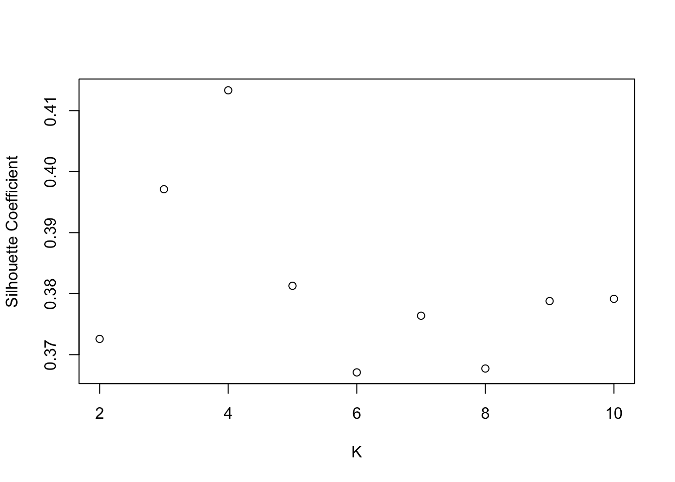
## [1] 0.3705446#Plotting silhouette vs K
plot.sil=function(data,max.K,max.iter,epsilon,dmatrix){
sil.vect=1:max.K
for(K in 2:max.K){
iter=min(max.iter,min.rep(K,epsilon))
kmeans.temp=repeat.kmeans(data,K,iter)
sil.vect[K]=mysil(kmeans.temp$cluster,dmatrix)
}
sil.vect=sil.vect[2:max.K]
plot(2:max.K,sil.vect,xlab="K",ylab="Silhouette Coefficient")
return(max(sil.vect))
}
plot.sil(mydata,10,1000,.01,dmatrix)
## [1] 0.835637910.1.3 Significance Test
## [1] 300## x y
## [1,] 1.820006 7.554873
## [2,] 16.944999 22.640867n=nrow(mydata)
range.matrix=apply(mydata,2,range)
u.x=runif(n,range.matrix[1,1],range.matrix[2,1])
u.y=runif(n,range.matrix[1,2],range.matrix[2,2])
udata=data.frame(u.x,u.y)
nrow(udata)## [1] 300## u.x u.y
## [1,] 1.821947 7.595441
## [2,] 16.875861 22.609389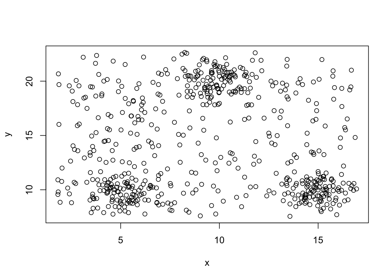
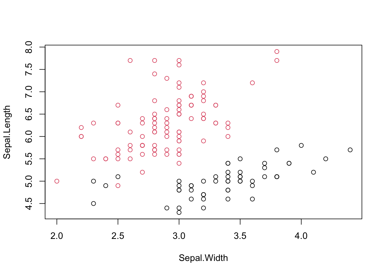
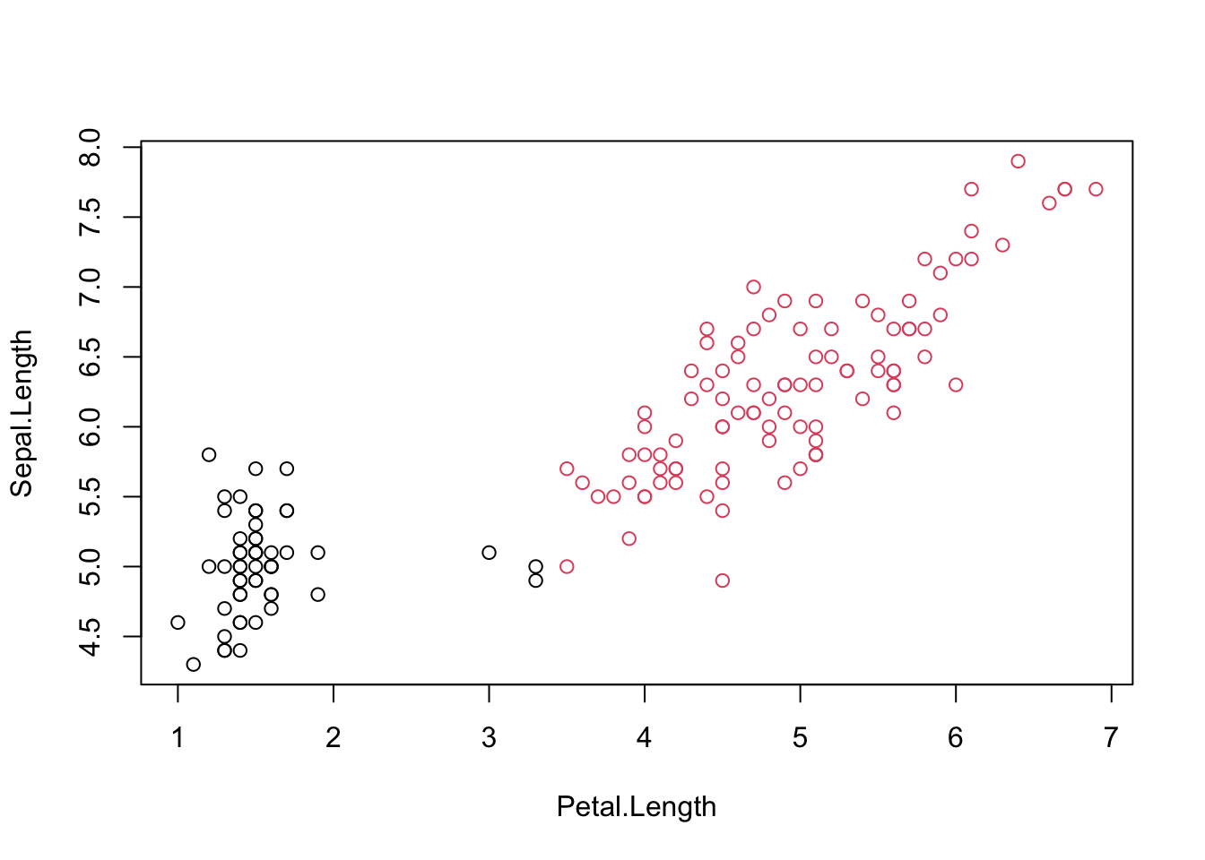
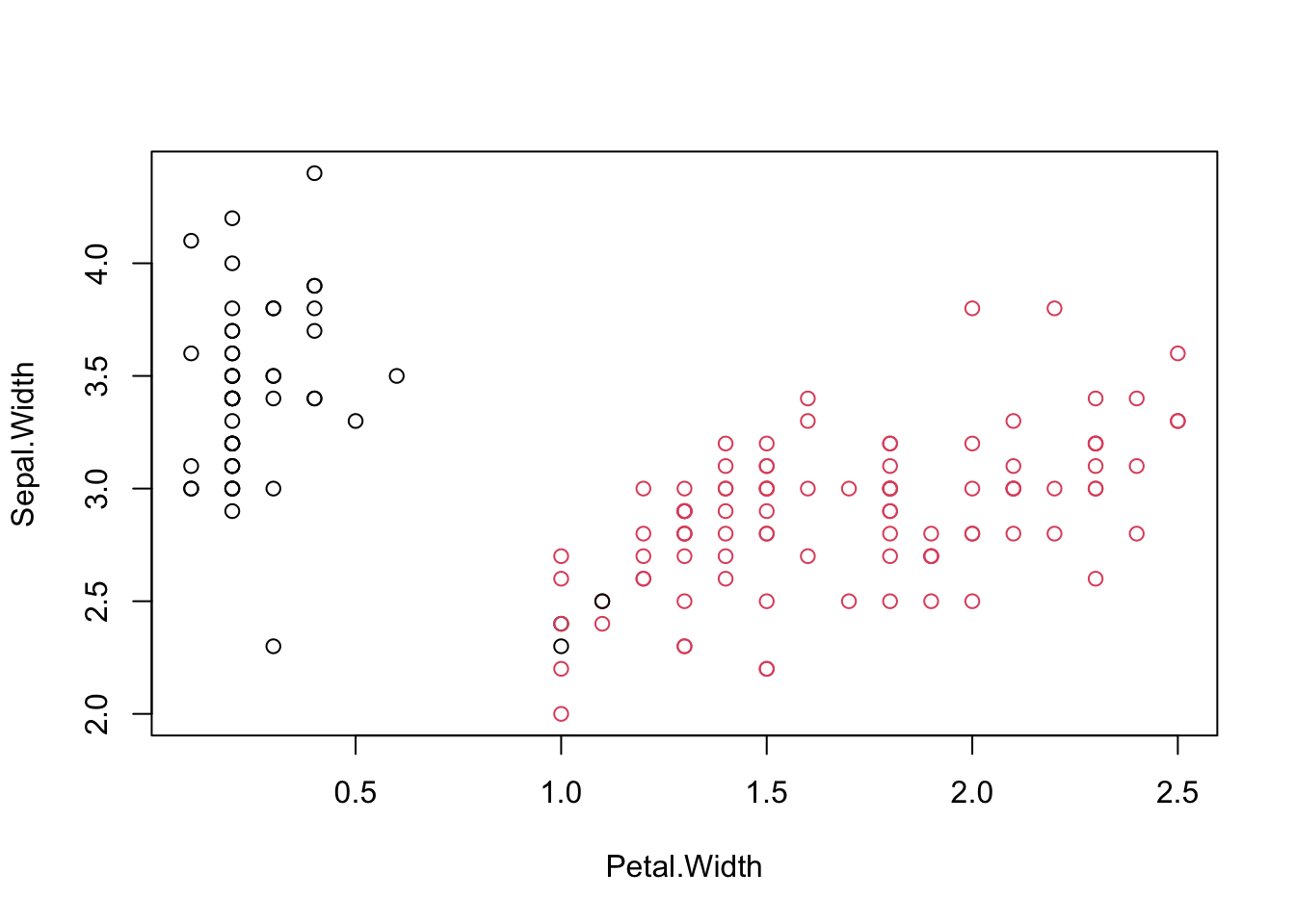
## [1] 0.4133293iris revisited
SSW and silhouette plots. Optimal K=2
## Warning: did not converge in 10 iterations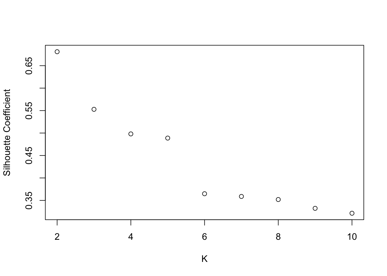
## [1] 0.6810462#Visualizing clusters
iris.kmeans=repeat.kmeans(iris.x,2,1000)
table(iris$Species,iris.kmeans$cluster)##
## 1 2
## setosa 50 0
## versicolor 3 47
## virginica 0 50


#Entropy for iris clustering
entropyterm=function(p){
  if(p==0){return(0)}
  return(-p*log(p,base=2))
}

entropy=function(p){
  return(sum(sapply(p,entropyterm)))
}

table.entropy=function(table){
  col.sums=apply(table,2,sum)
  col.props=col.sums/sum(col.sums)
  for(j in 1:ncol(table)){
    if(sum(table[,j]!=0)){
      table[,j]=table[,j]/sum(table[,j])
    }
  }
  table.entropies=apply(table,2,entropy)
  return(col.props%*%table.entropies)
}

iris.table=table(iris$Species,
                 iris.kmeans$cluster)
table.entropy(iris.table)
## [,1]
## [1,] 0.757101CHI-SQUARE TEST OF INDEPENDENCE
##      [,1] [,2] [,3] [,4]
## [1,]   16   14   13   13
## [2,] 14 6 10 8##
## Pearson's Chi-squared test
##
## data: mytable
## X-squared = 1.5242, df = 3, p-value = 0.6767## [1] 0.6776621##
## Pearson's Chi-squared test with simulated p-value (based on 2000 replicates)
##
## data: mytable
## X-squared = 1.5242, df = NA, p-value = 0.6697#Testing independence of clusters
#and Species labels for iris data
iris.x=iris[,1:4]
iris.kmeans=repeat.kmeans(iris.x,2,1000)
iris.table=table(iris$Species,
iris.kmeans$cluster)
chisq.test(iris.table,simulate.p.value=TRUE)##
## Pearson's Chi-squared test with simulated p-value (based on 2000 replicates)
##
## data: iris.table
## X-squared = 137.66, df = NA, p-value = 0.0004998##
## Pearson's Chi-squared test
##
## data: iris.table
## X-squared = 137.66, df = 2, p-value < 2.2e-1610.1.4 DBSCAN
Creating some data
unif.rect function
unif.rect=function(n,x0,y0,deltax,deltay){
  x=runif(n,x0,x0+deltax)
  y=runif(n,y0,y0+deltay)
  return(cbind(x,y))
}

mydata=unif.rect(500,5,7,15,23)
plot(mydata,asp=1)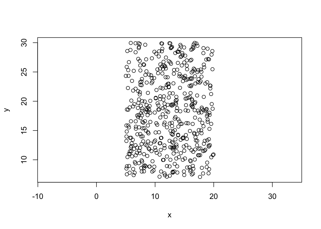
#mydata1
mydata1=rbind(unif.rect(5*n,0,0,1,5),
             unif.rect(4*n,1,0,4,1),
             unif.rect(4*n,4,1,1,4))
plot(mydata1,asp=1)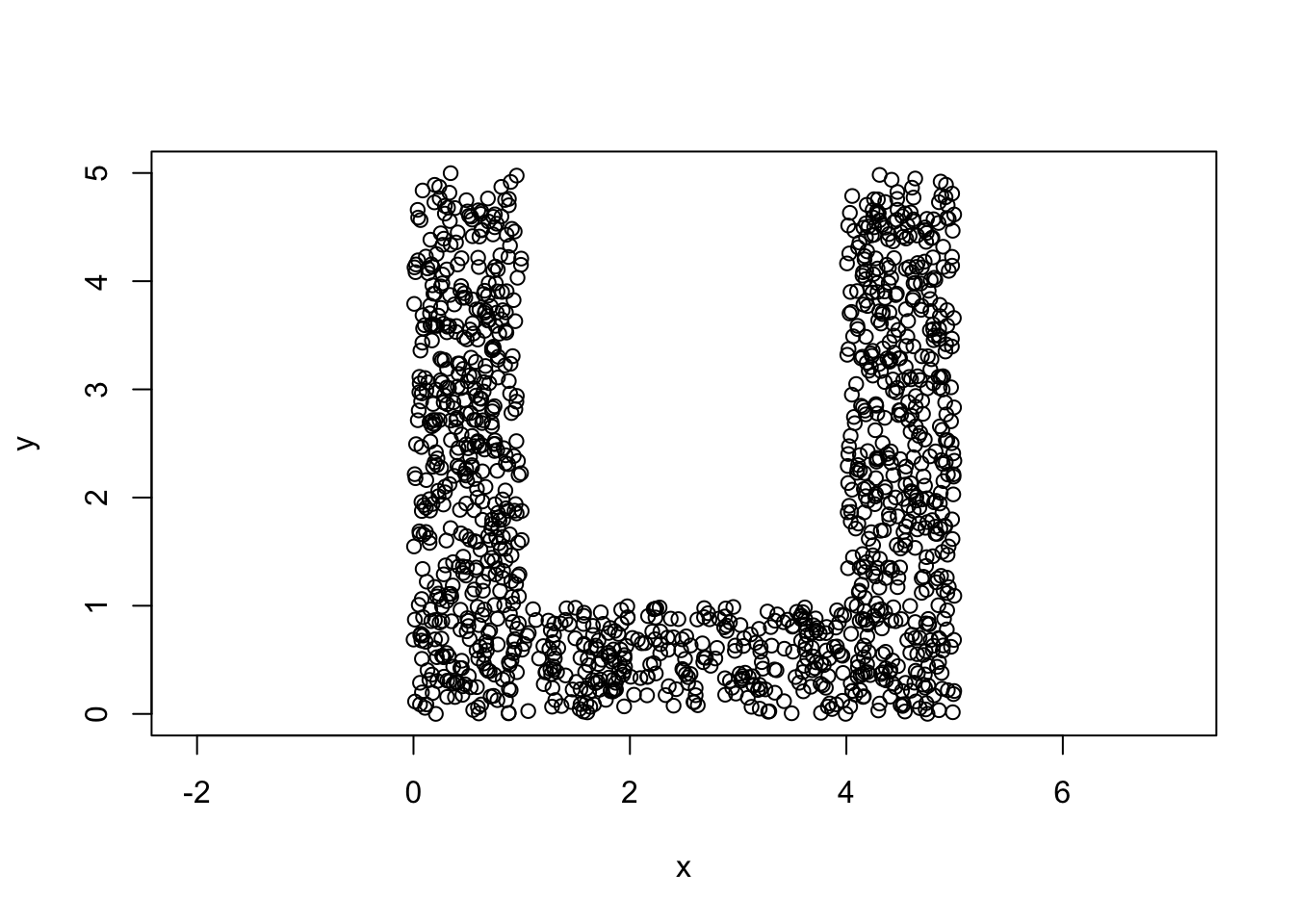
#mydata2
temp=rbind(unif.rect(5*n,0,0,1,5),
           unif.rect(4*n,1,0,4,1),
           unif.rect(4*n,4,1,1,4))
mydata2=temp%*%cbind(c(1,0),c(0,-1))+cbind(rep(2,13*n),rep(7,13*n))
plot(mydata2,asp=1)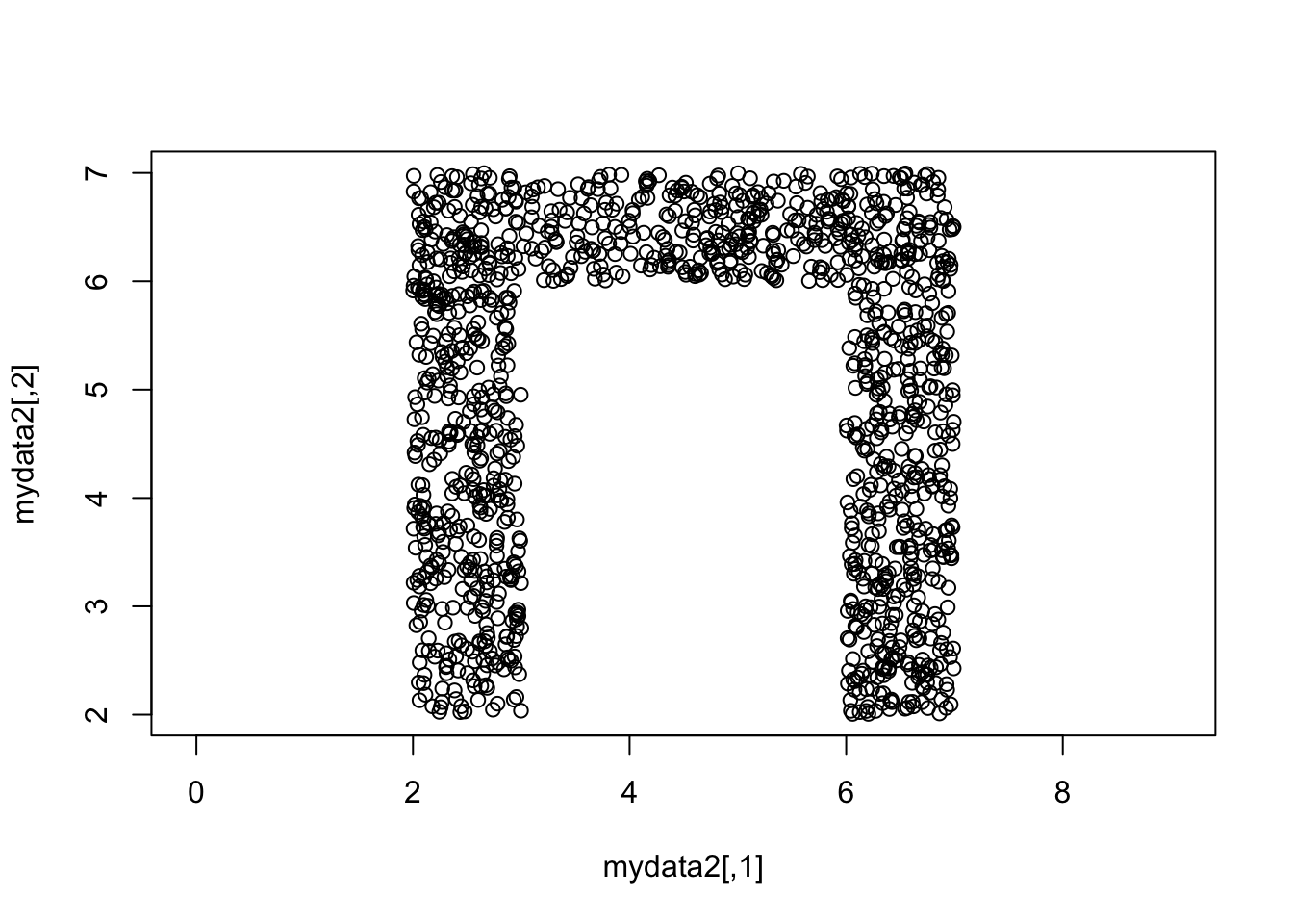
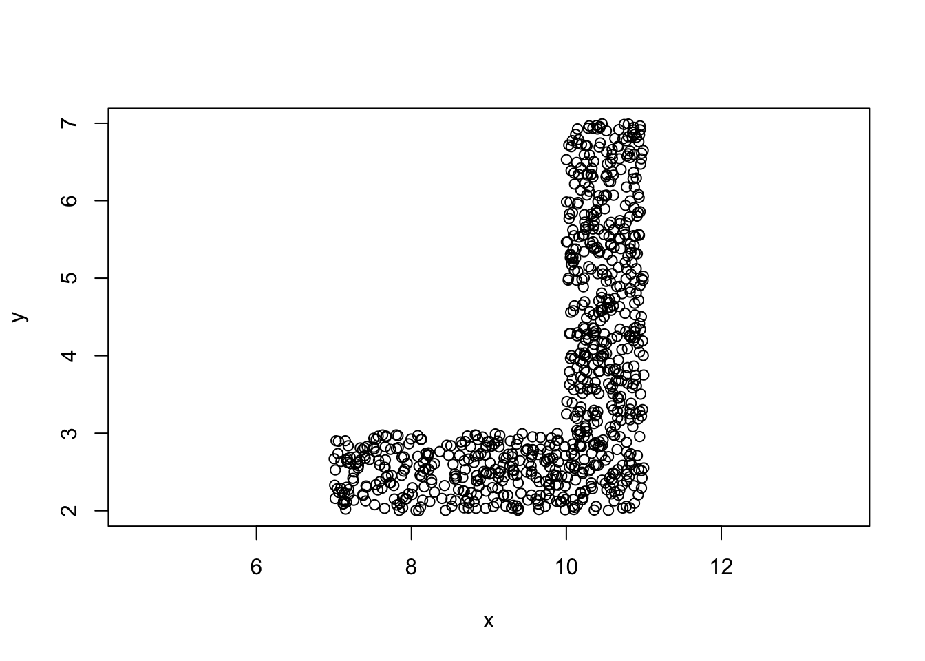
#mydata4
temp=rbind(unif.rect(5*n,0,0,1,5),
           unif.rect(4*n,1,0,4,1),
           unif.rect(4*n,4,1,1,4))
mydata4=temp%*%cbind(c(1,0),c(0,-1))+cbind(rep(8,13*n),rep(9,13*n))
plot(mydata4,asp=1)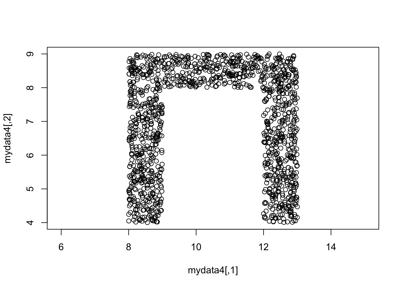
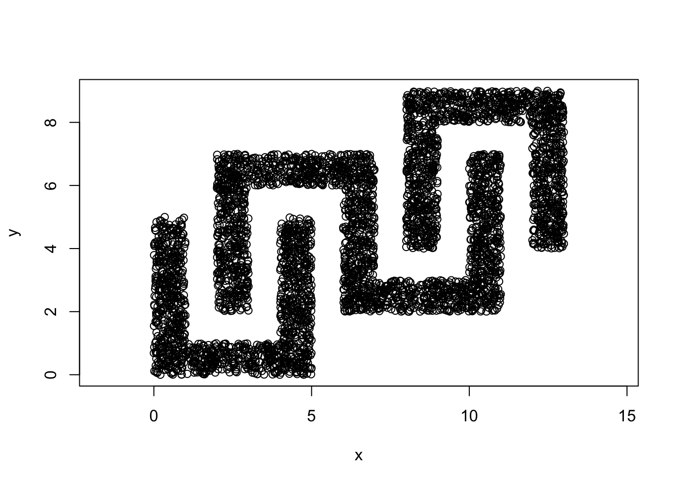
#Adding noise
m=round(.08*47*n,0)
mydata5=cbind(runif(m,0,13),
              runif(m,0,9))

mydata=rbind(mydata,
             mydata5)
plot(mydata,asp=1)
DBSCAN
## [1] "cluster" "eps" "MinPts" "isseed"## [1] 1 1 1 1 1 1 1 1 1 1 1 1 1 1 1 1 1 1 1 1 1 1 1 1 1 1 1 1 1 1 1 1 1 1 1 1 1 1 1 1 1 1 1 1 1 1 1
## [48] 1 1 1 1 1 1 1 1 1 1 1 1 1 1 1 1 1 1 1 1 1 1 1 1 1 1 1 1 1 1 1 1 1 1 1 1 1 1 1 1 1 1 1 1 1 1 1
## [95] 1 1 1 1 1 1 1 1 1 1 1 1 1 1 1 1 1 1 1 1 1 1 1 1 1 1 1 1 1 1 1 1 1 1 1 1 1 1 1 1 1 1 1 1 1 1 1
## [142] 1 1 1 1 1 1 1 1 1 1 1 1 1 1 1 1 1 1 1 1 1 1 1 1 1 1 1 1 1 1 1 1 1 1 1 1 1 1 1 1 1 1 1 1 1 1 1
## [189] 1 1 1 1 1 1 1 1 1 1 1 1 1 1 1 1 1 1 1 1 1 1 1 1 1 1 1 1 1 1 1 1 1 1 1 1 1 1 1 1 1 1 1 1 1 1 1
## [236] 1 1 1 1 1 1 1 1 1 1 1 1 1 1 1 1 1 1 1 1 1 1 1 1 1 1 1 1 1 1 1 1 1 1 1 1 1 1 1 1 1 1 1 1 1 1 1
## [283] 1 1 1 1 1 1 1 1 1 1 1 1 1 1 1 1 1 1 1 1 1 1 1 1 1 1 1 1 1 1 1 1 1 1 1 1 1 1 1 1 1 1 1 1 1 1 1
## [330] 1 1 1 1 1 1 1 1 1 1 1 1 1 1 1 1 1 1 1 1 1 1 1 1 1 1 1 1 1 1 1 1 1 1 1 1 1 1 1 1 1 1 1 1 1 1 1
## [377] 1 1 1 1 1 1 1 1 1 1 1 1 1 1 1 1 1 1 1 1 1 1 1 1 1 1 1 1 1 1 1 1 1 1 1 1 1 1 1 1 1 1 1 1 1 1 1
## [424] 1 1 1 1 1 1 1 1 1 1 1 1 1 1 1 1 1 1 1 1 1 1 1 1 1 1 1 1 1 1 1 1 1 1 1 1 1 1 1 1 1 1 1 1 1 1 1
## [471] 1 1 1 1 1 1 1 1 1 1 1 1 1 1 1 1 1 1 1 1 1 1 1 1 1 1 1 1 1 1 1 1 1 1 1 1 1 1 1 1 1 1 1 1 1 1 1
## [518] 1 1 1 1 1 1 1 1 1 1 1 1 1 1 1 1 1 1 1 1 1 1 1 1 1 1 1 1 1 1 1 1 1 1 1 1 1 1 1 1 1 1 1 1 1 1 1
## [565] 1 1 1 1 1 1 1 1 1 1 1 1 1 1 1 1 1 1 1 1 1 1 1 1 1 1 1 1 1 1 1 1 1 1 1 1 1 1 1 1 1 1 1 1 1 1 1
## [612] 1 1 1 1 1 1 1 1 1 1 1 1 1 1 1 1 1 1 1 1 1 1 1 1 1 1 1 1 1 1 1 1 1 1 1 1 1 1 1 1 1 1 1 1 1 1 1
## [659] 1 1 1 1 1 1 1 1 1 1 1 1 1 1 1 1 1 1 1 1 1 1 1 1 1 1 1 1 1 1 1 1 1 1 1 1 1 1 1 1 1 1 1 1 1 1 1
## [706] 1 1 1 1 1 1 1 1 1 1 1 1 1 1 1 1 1 1 1 1 1 1 1 1 1 1 1 1 1 1 1 1 1 1 1 1 1 1 1 1 1 1 1 1 1 1 1
## [753] 1 1 1 1 1 1 1 1 1 1 1 1 1 1 1 1 1 1 1 1 1 1 1 1 1 1 1 1 1 1 1 1 1 1 1 1 1 1 1 1 1 1 1 1 1 1 1
## [800] 1 1 1 1 1 1 1 1 1 1 1 1 1 1 1 1 1 1 1 1 1 1 1 1 1 1 1 1 1 1 1 1 1 1 1 1 1 1 1 1 1 1 1 1 1 1 1
## [847] 1 1 1 1 1 1 1 1 1 1 1 1 1 1 1 1 1 1 1 1 1 1 1 1 1 1 1 1 1 1 1 1 1 1 1 1 1 1 1 1 1 1 1 1 1 1 1
## [894] 1 1 1 1 1 1 1 1 1 1 1 1 1 1 1 1 1 1 1 1 1 1 1 1 1 1 1 1 1 1 1 1 1 1 1 1 1 1 1 1 1 1 1 1 1 1 1
## [941] 1 1 1 1 1 1 1 1 1 1 1 1 1 1 1 1 1 1 1 1 1 1 1 1 1 1 1 1 1 1 1 1 1 1 1 1 1 1 1 1 1 1 1 1 1 1 1
## [988] 1 1 1 1 1 1 1 1 1 1 1 1 1
## [ reached getOption("max.print") -- omitted 4076 entries ]

#Determining Eps

dmatrix=rdist(mydata)
sort.dmatrix=apply(dmatrix,2,sort)

#k-dist means distance to
#kth nearest neighbor

k=5
kdist=sort.dmatrix[k,]

plot(sort(kdist),type="l",
     xlab="Points Sorted by k-dist",
     ylab="k-dist")
lines(1:length(kdist),rep(0.2,length(kdist)),col="red")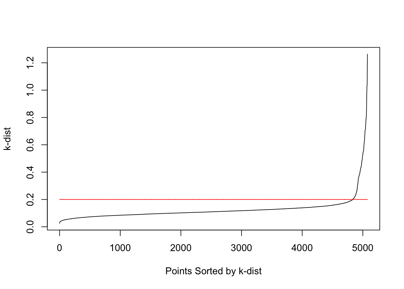
#Eps too large
mydata.dbscan=dbscan(mydata,eps=0.6,MinPts=5)
plot(mydata,asp=1,col=(mydata.dbscan$cluster+1))
#Eps too small
mydata.dbscan=dbscan(mydata,eps=0.1,MinPts=5)
plot(mydata,asp=1,col=(mydata.dbscan$cluster+1))
DBSCAN for iris data
#Standardizing iris
x=iris[,1:4]
xbar=apply(x,2,mean)
xbarMatrix=cbind(rep(1,150))%*%xbar
s=apply(x,2,sd)
sMatrix=cbind(rep(1,150))%*%s

z=(x-xbarMatrix)/sMatrix
apply(z,2,mean)
## Sepal.Length Sepal.Width Petal.Length Petal.Width
## -4.484318e-16 2.034094e-16 -2.895326e-17 -2.989362e-17## Sepal.Length Sepal.Width Petal.Length Petal.Width
## 1 1 1 1
#Determining Eps

dmatrix=rdist(z)
sort.dmatrix=apply(dmatrix,2,sort)

k=5
kdist=sort.dmatrix[k,]

plot(sort(kdist),type="l",
     xlab="Points Sorted by k-dist",
     ylab="k-dist")
lines(1:length(kdist),rep(0.79,length(kdist)),col="red")

##
##  0  1  2
## 4 49 97##
## 1 2
## setosa 49 0
## versicolor 0 50
## virginica 0 47##
## Pearson's Chi-squared test with simulated p-value (based on 2000 replicates)
##
## data: iris.table
## X-squared = 146, df = NA, p-value = 0.000499810.1.5 Agglomerative Hierarchical Clustering
Generating some data
x1=c(0,1,-2)
y1=c(0,1,3)
mydata1=cbind(x1,y1)

x2=c(0,3,1.5)
y2=c(0,0,-8)
mydata2=cbind(10+x2,y2)

x3=c(0,0,1)
y3=c(0,1,-5)
mydata3=cbind(5+x3,20+y3)

mydata=rbind(mydata1,mydata2,mydata3)
plot(mydata)

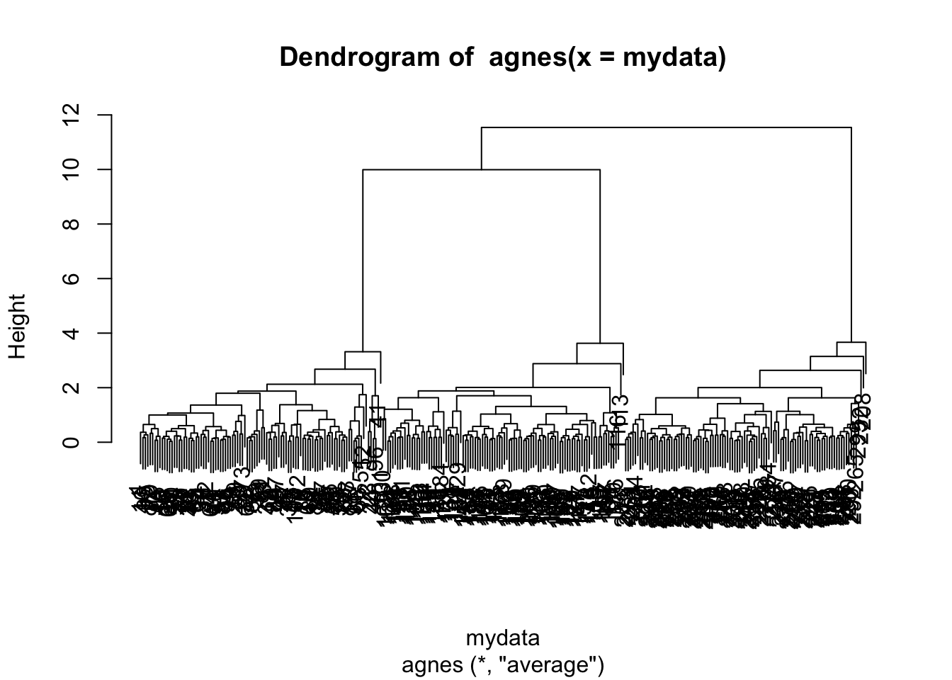
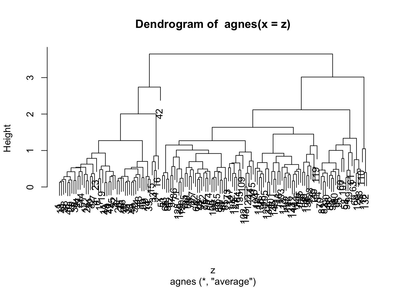
#agnes (Agglomerative Nesting)
library(cluster)

mydata.agnes=agnes(mydata)


#dendrogram
pltree(mydata.agnes)
## [1] 1.000000 1.414214 3.000000 3.605551 5.590891 8.139410 13.001741 20.308999cutting the tree at a given height
mydata.cluster=cutree(as.hclust(mydata.agnes), h = 10)
plot(mydata,col=mydata.cluster,pch=as.character(row.num))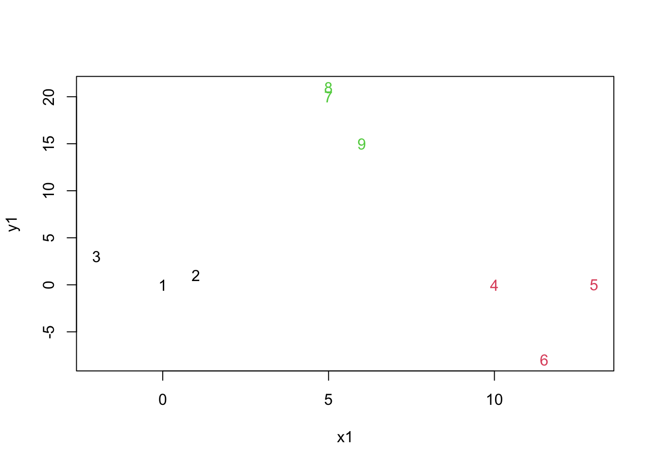
mydata.cluster=cutree(as.hclust(mydata.agnes), h = 15)
plot(mydata,col=mydata.cluster,pch=as.character(row.num))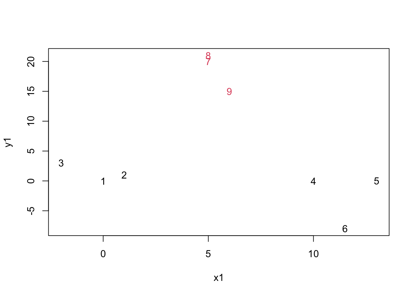
mydata.heights=sort(mydata.agnes$height)
mydata.cluster=cutree(as.hclust(mydata.agnes), h = mydata.heights[2])
plot(mydata,col=mydata.cluster,pch=as.character(row.num))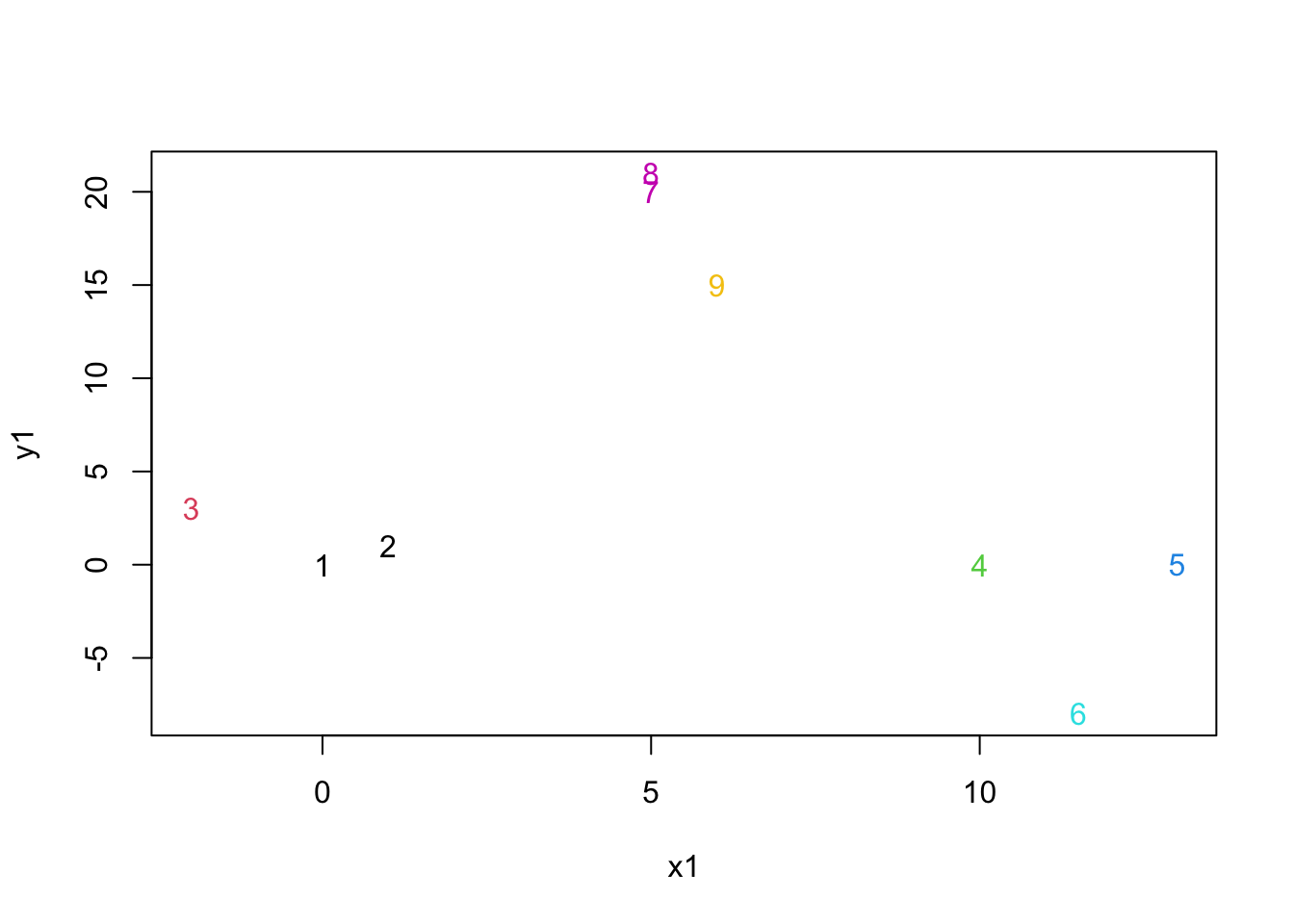
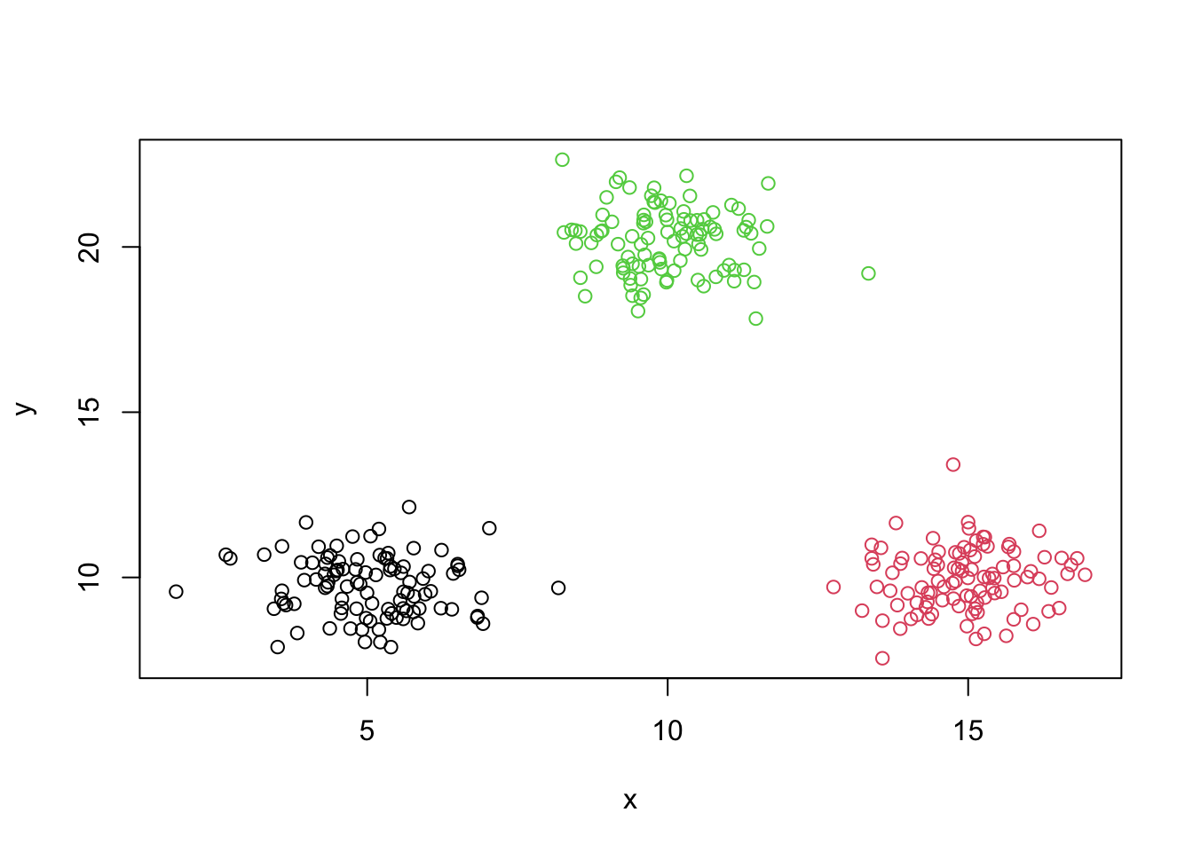
#cutting the tree based on number of clusters

mydata.cluster=cutree(as.hclust(mydata.agnes), k = 4)
plot(mydata,col=mydata.cluster,pch=as.character(row.num))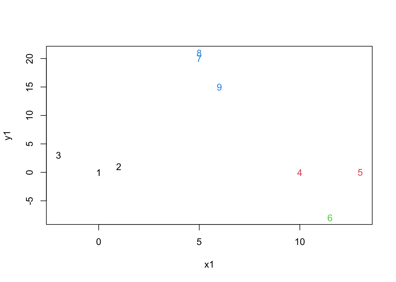
mydata.cluster=cutree(as.hclust(mydata.agnes), k = 2)
plot(mydata,col=mydata.cluster,pch=as.character(row.num))
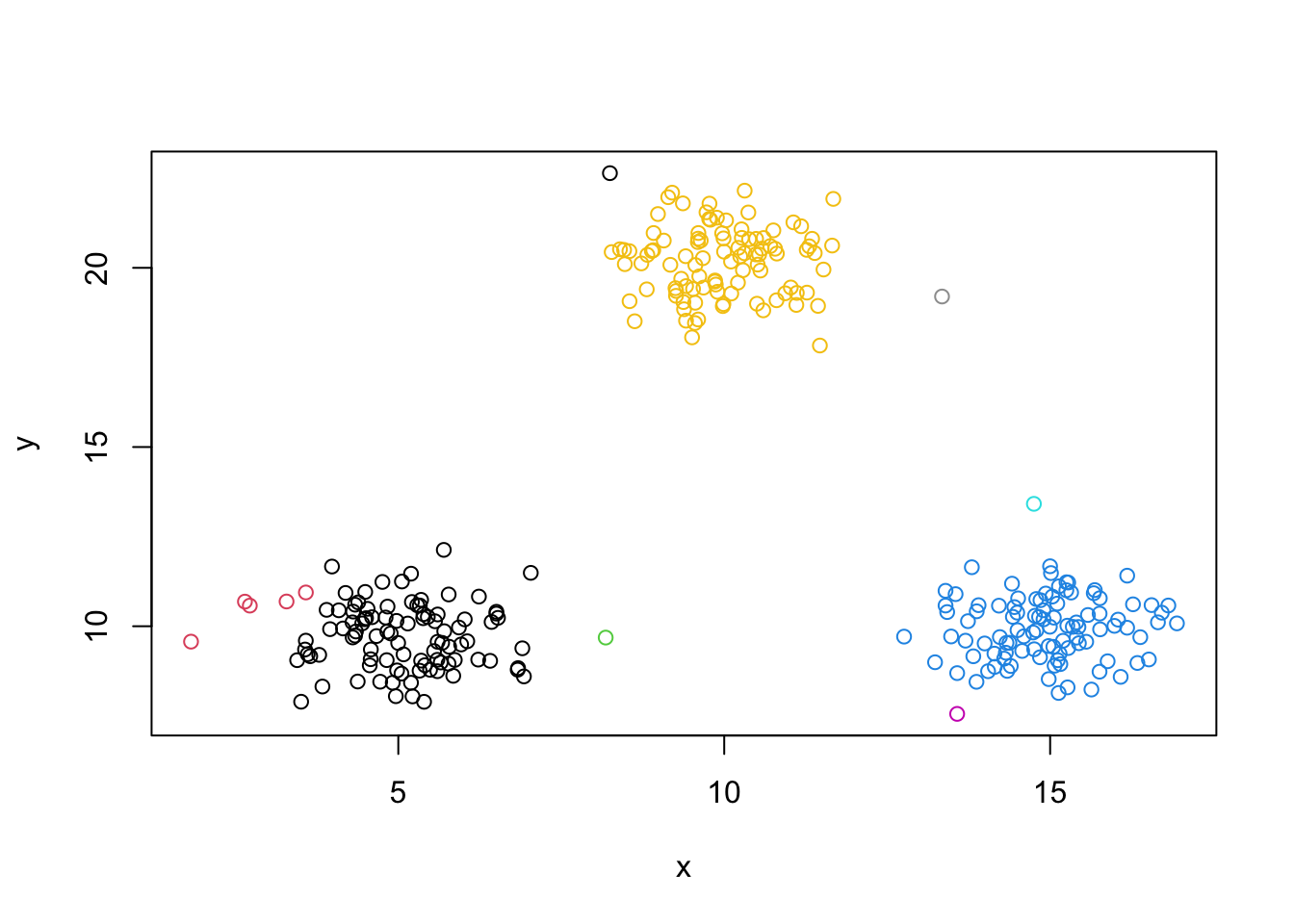
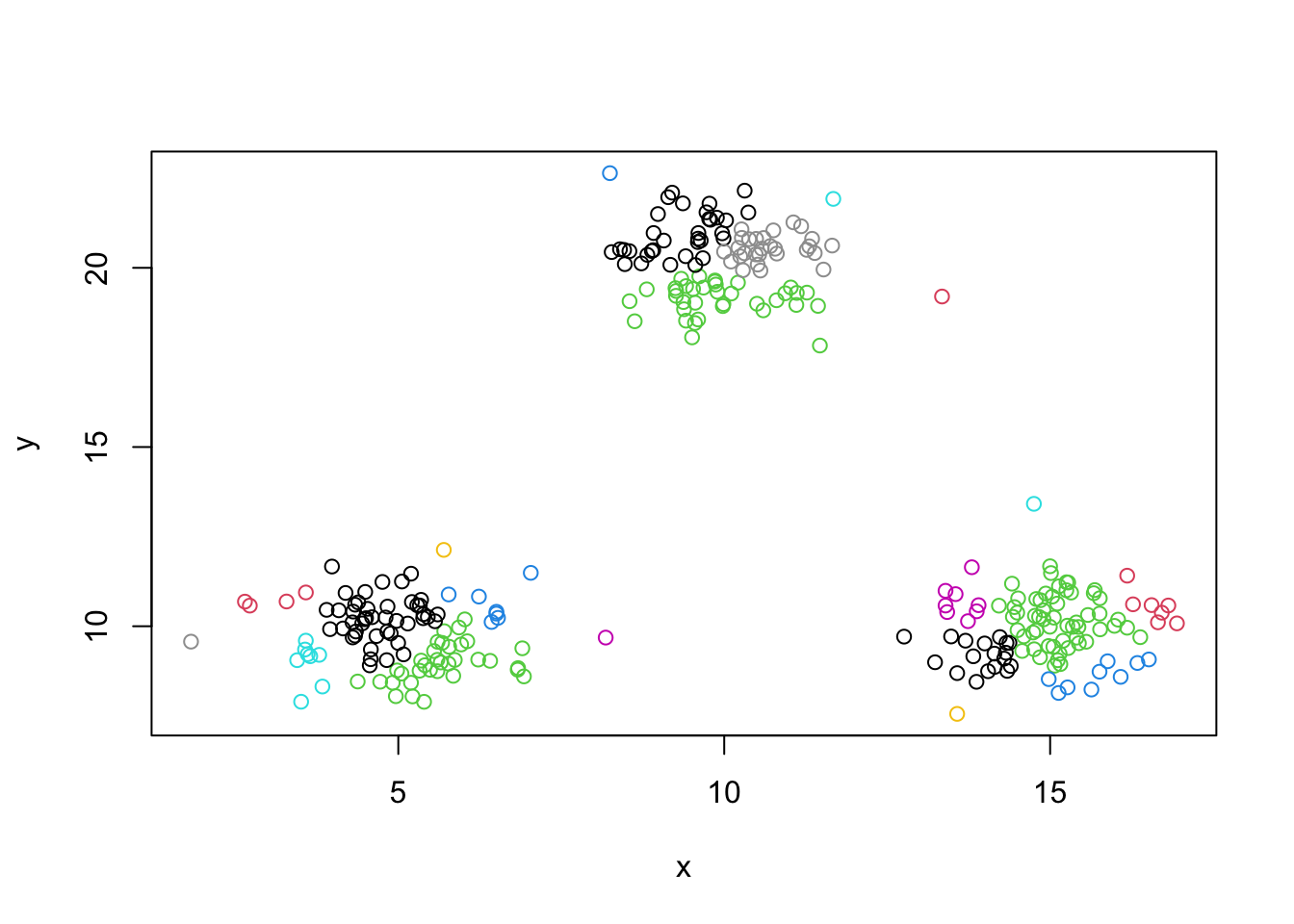
mydata.cluster=cutree(as.hclust(mydata.agnes), k = 7)
plot(mydata,col=mydata.cluster,pch=as.character(row.num))
#Generating some data
set.seed(5364)
x1=rnorm(100,5,1)
x2=rnorm(100,15,1)
x3=rnorm(100,10,1)

y1=rnorm(100,10,1)
y2=rnorm(100,10,1)
y3=rnorm(100,20,1)

mydata=data.frame(x=c(x1,x2,x3),y=c(y1,y2,y3))
plot(y~x,data=mydata,asp=1)
iris data
Standardizing iris
x=iris[,1:4]
xbar=apply(x,2,mean)
xbarMatrix=cbind(rep(1,150))%*%xbar
s=apply(x,2,sd)
sMatrix=cbind(rep(1,150))%*%s

z=(x-xbarMatrix)/sMatrix
apply(z,2,mean)
## Sepal.Length Sepal.Width Petal.Length Petal.Width
## -4.484318e-16 2.034094e-16 -2.895326e-17 -2.989362e-17## Sepal.Length Sepal.Width Petal.Length Petal.Width
## 1 1 1 1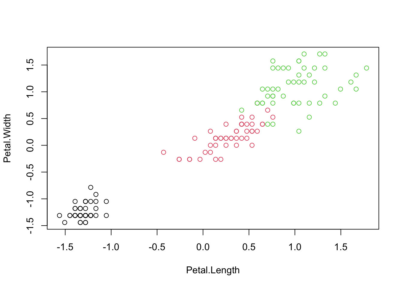

##             iris.cluster
##               1  2
##   setosa     50  0
##   versicolor  0 50
##   virginica   0 50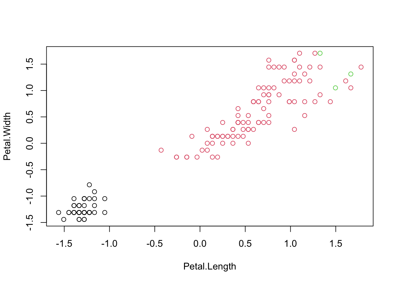
##             iris.cluster
##               1  2  3
##   setosa     50  0  0
##   versicolor  0 50  0
##   virginica   0 47  3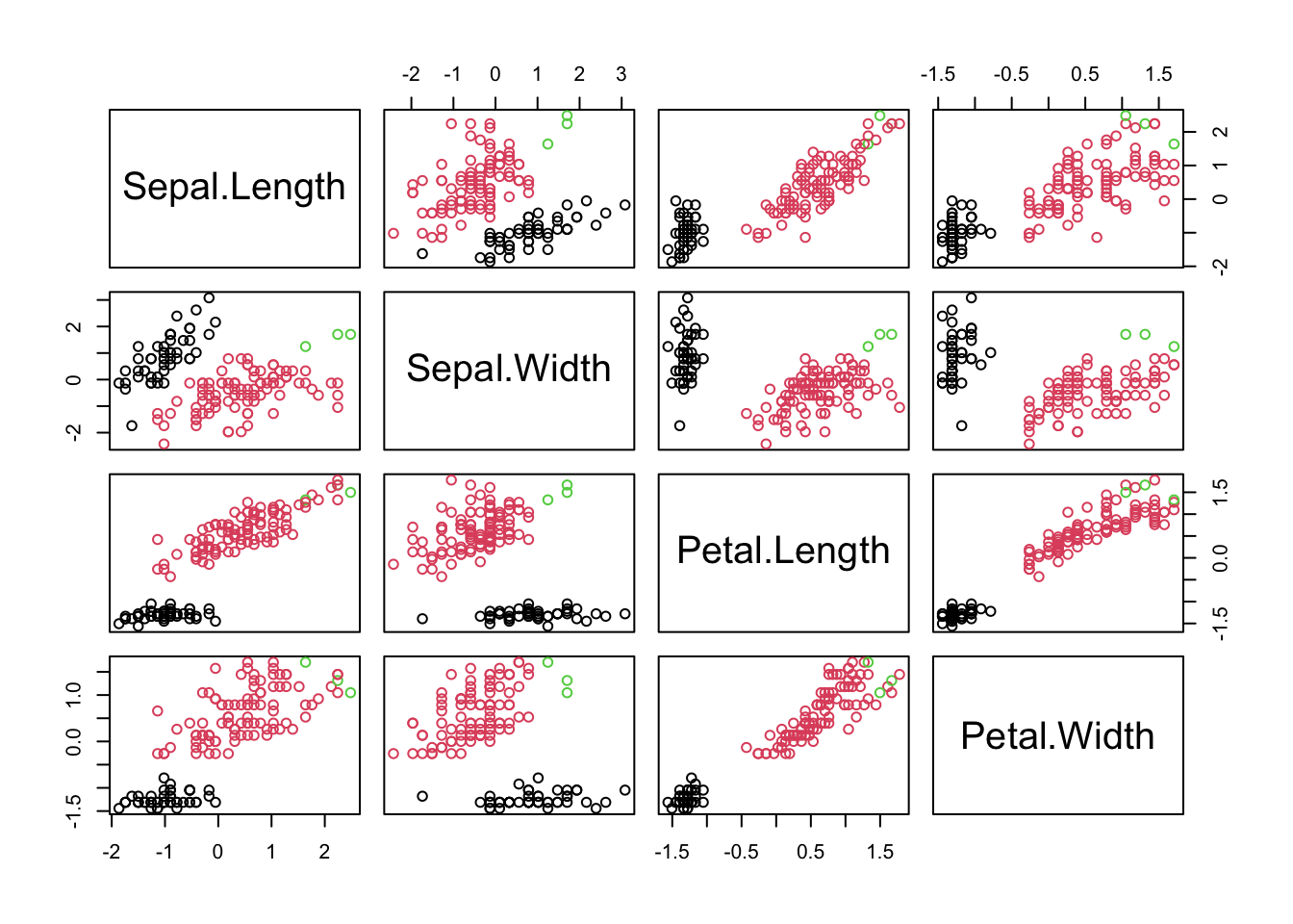
##             iris.cluster
##               1  2  3  4  5  6  7  8  9 10
##   setosa     28 17  4  1  0  0  0  0  0  0
##   versicolor  0  0  0  0 30 16  3  1  0  0
##   virginica   0  0  0  0 15  1  1 22  8  3
10.1.6 GAUSSIAN MIXTURE EM CLUSTERING
#Generating data
set.seed(5364)
x1=rnorm(100,5,1)
x2=rnorm(100,15,1)
x3=rnorm(100,10,1)

y1=rnorm(100,10,1)
y2=rnorm(100,10,1)
y3=rnorm(100,20,1)

mydata=data.frame(x=c(x1,x2,x3),y=c(y1,y2,y3))
plot(y~x,data=mydata,asp=1)
## number of iterations= 4## [1] "x" "lambda" "mu" "sigma" "loglik" "posterior" "all.loglik"
## [8] "restarts" "ft"#Posterior probabilities and clusters
#mydata.gauss$posterior
mydata.cluster=apply(mydata.gauss$posterior,
1,
which.max)
plot(mydata,col=mydata.cluster)
#Prior probabilities (also called mixing probabilities)
mydata.gauss$lambda## [1] 0.3333333 0.3333333 0.3333333## [[1]]
## [1] 5.030316 9.750965
##
## [[2]]
## [1] 14.935464 9.941784
##
## [[3]]
## [1] 9.986731 20.181994points(rbind(mydata.gauss$mu[[1]],
mydata.gauss$mu[[2]],
mydata.gauss$mu[[3]]),
pch=24,bg='blue',col="blue")
## [[1]]
##             [,1]        [,2]
## [1,]  1.07638821 -0.07027661
## [2,] -0.07027661  0.80296445
##
## [[2]]
##            [,1]       [,2]
## [1,] 0.78745014 0.07154876
## [2,] 0.07154876 0.86209277
##
## [[3]]
##             [,1]        [,2]
## [1,]  0.83455170 -0.06130202
## [2,] -0.06130202  0.96382845
Generating more data
multi.rnorm returns an n x p matrix, whose rows are randomly generated normal random vectors with mean vector mu and covariance matrix Sigma
##      [,1] [,2]
## [1,]   25    8
## [2,] 8 16## [,1] [,2]
## [1,] 4.9168996 0.9077988
## [2,] 0.9077988 3.8956259## [,1] [,2]
## [1,] 25 8
## [2,] 8 16multi.rnorm=function(n,mu,Sigma){
p=length(mu)
Z=matrix(nrow=n,
ncol=p,
rnorm(n*p))
X=rep(1,n)%*%rbind(mu)+Z%*%sqrtm(Sigma)
return(X)
}
mu=c(5,10)
Sigma=cbind(c(25,8),c(8,16))
X=multi.rnorm(1000000,mu,Sigma)
apply(X,2,mean)## [1] 4.992743 9.996079## [,1] [,2]
## [1,] 24.992858 7.975951
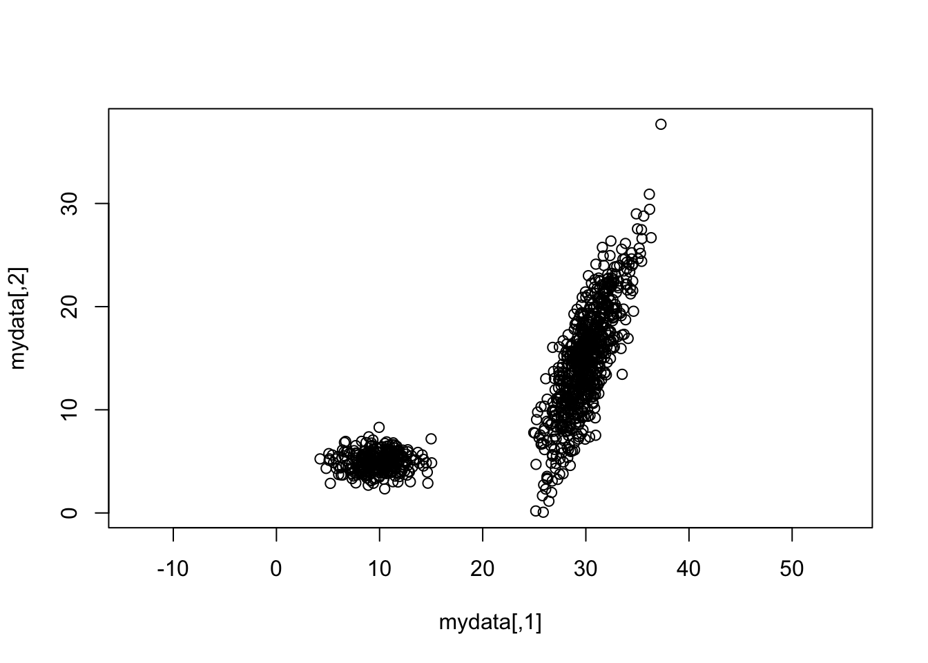
## [2,] 7.975951 15.959923Another example
mu1=c(10,5)
Sigma1=cbind(c(4,0),c(0,1))

mu2=c(30,15)
Sigma2=cbind(c(4,8),c(8,25))


mydata=rbind(multi.rnorm(300,mu1,Sigma1),
             multi.rnorm(700,mu2,Sigma2))

plot(mydata,asp=1)