Chapter 1 R Review
There are many introduction to R tutoraials. Hence, here we will only provide a very quick introduction to R.
Getting Started
- Download R from https://cloud.r-project.org/ (or any other sources/ package managers)
- Download R-Studio from https://rstudio.com/products/rstudio/download/#download
R is the underlying programming language and R-studio is the friendly GUI editor (IDE). Usually, the R-studio screen is divided into four sections called ‘panes’. We can write our code on source where we can save them in a file, known as script and we can run that script in the console. This way, R-Studio provides a very friendly way to interact with R.
When we talk about R, there are two parts. First part is the base R, which are the pre built R data structures and functions. The second part is the added R functionality generated by installing packages from other R users. To simplify, packages are bundled R (or other language) code bundled so that we can simply reuse them. Base R has many useful functions and can be extended by using additional R packages.
When we work in R, we usually work with data. Data can be loaded in R from external files, internet, database, created in R, or be loaded from R packages themselves. Some famous dataset is already available in R or R packages which we will see later.
R can understand following data structure by default and can do mathematical operations. Anything beginning with a # is a comment and will be ignored by R while running the code. We can write comments to write notes about the code.
- Numeric or Integer : data type that represents a value which can be continuous or discrete
- String: letters and words
- Factor: category
- Date and Time: date and time
- Boolean: TRUE or FALSE
Using these, we can do from simple arithematic to very complicated deep learning in R.
1.1 Basic Arithematic, vectors and Matrices
## [1] 4## [1] 3## [1] 28## [1] 2.333333## [1] 8## [1] 5## [1] 25Working with vectors in R
## [1] 7 9 3 -8 5## [1] 7## [1] -8## [1] 3 4 5 6 7 8 9## [1] 15 15 15 15## [1] 7 9 11 13 15## [1] 1 2 3 4 5 6 7 8 9 10## [1] 5## [1] 10## [1] 6 14 24 36 50## [1] 1 4 9 16 25## [1] 0.1666667 0.2857143 0.3750000 0.4444444 0.5000000Working with Matrices in R
We can create a matrix by combining vectors
##      x y z
## [1,] 1 4 7
## [2,] 2 5 8
## [3,] 3 6 9## [,1] [,2]
## [1,] 10 50
## [2,] 11 51
## [3,] 12 52# creating matrix with same element as B but differnt order
C=matrix(c(10,11,12,50,51,52),3,2,byrow='true')
C## [,1] [,2]
## [1,] 10 11
## [2,] 12 50
## [3,] 51 52Doing matrix operation in R
#Matrix multiplication in R is given by %*%.

A=matrix(1:4,2,2,byrow='true')
B=matrix(5:8,2,2,byrow='true')
A
## [,1] [,2]
## [1,] 1 2
## [2,] 3 4## [,1] [,2]
## [1,] 5 6
## [2,] 7 8## [,1] [,2]
## [1,] 6 8
## [2,] 10 12## [,1] [,2]
## [1,] 5 12
## [2,] 21 32## [,1] [,2]
## [1,] 19 22
## [2,] 43 50## [,1] [,2]
## [1,] 1 4
## [2,] 9 16## [,1] [,2]
## [1,] 8 9
## [2,] 10 11## [,1] [,2]
## [1,] 7 10
## [2,] 15 22## [,1] [,2]
## [1,] 1 3
## [2,] 2 4## [1] 1 4## [,1] [,2] [,3]
## [1,] 1 0 0
## [2,] 0 1 0
## [3,] 0 0 1## [,1] [,2]
## [1,] 1.0000000 0.50
## [2,] 0.3333333 0.25## [,1] [,2]
## [1,] -2.0 1.0
## [2,] 1.5 -0.5## [,1] [,2]
## [1,] 1.000000e+00 0
## [2,] 1.110223e-16 11.2 Programming in R
Using Control flow
IF ELSE
## [1] "Yes, it is."## [1] "Yes, it is."## [1] "No, it is not"Loops
## [1] 1 1 1 1 1 1 1 1 1 1## [1] 1 4 9 16 25 36 49 64 81 100Creating custom functions
Simple function that adds two number
## [1] 8List is an special object in R. Functions with list capacity
#The next function uses an R object called a list.  Here's an example to
#show how lists work.

L=list(x=5,y=1:4,z=diag(7))

L$x
## [1] 5## [1] 1 2 3 4## [,1] [,2] [,3] [,4] [,5] [,6] [,7]
## [1,] 1 0 0 0 0 0 0
## [2,] 0 1 0 0 0 0 0
## [3,] 0 0 1 0 0 0 0
## [4,] 0 0 0 1 0 0 0
## [5,] 0 0 0 0 1 0 0
## [6,] 0 0 0 0 0 1 0
## [7,] 0 0 0 0 0 0 1myops=function(x,y){
mysum=x+y
mydiff=x-y
myprod=x*y
myquot=x/y
list(sum=mysum,diff=mydiff,prod=myprod,quot=myquot)
}
myops(5,3)$sum## [1] 8## [1] 2## [1] 15## [1] 1.6666671.3 Simulating Data in R
Data can be simulated in R in different ways on case by case basis. We can generate data to follow certain structure by using functions in R. Function in R can be identified by the parenthesis. For example, lets look at this line x <- seq(from=1, to=10). Here x is the name of the ‘variable’, the value the output of the function takes so that we can use it later. <- is an assignment operator which is assigning the result of the right side to the variable named on left. In R, we could use <- or = interchangably. seq() is the sequence generation function, a way to create a sequence. The things inside the parenthesis are called parameters. It is very common to skip writing from= and to= when using the function since the parameters are accepted in the given order. If we do not understand what a the given sequence generation does we can ask for help by typing ?seq() [or ??seq() or help(seq)]. Understanding the help output can be challenging sometimes but fear not. It is an acquired skill
Try following codes.
# assigning values to x and y variables
x <- 1:10
y <- seq(1,10)

#checking if x and y are equal
x == y

# generating sequence but with different interval
z <- seq(0, 10, .1)

# squaring the values of z and assigning it to a variable
z_sq <- z^2
?seq()
There are many other ways to create data. For example, we can generate data data follows certain pattern. rnorm() creates normally distributed data centered on mean and runif() creates uniformly distributed data on a given interval.
If we want to see the output of the variable, we can type the name of the variable and hit enter. Alternatively we can use print() function with the variable as the “parameter”
1.4 R Datasets
We can think of a dataset a
Some famous datasets are available in R. Check them out by running data() function on the console.
Note: These data are from a particular package called datasets. There are more data in other packages (as you can see if you scroll the result from data() screen using data(package = .packages(all.available = TRUE))).
As you load more packages, you may get more R data. You can access dataset from particular package by telling which package you want to look at.
We can load a dataset into R and print first 6 rows of that dataset using head() function. Check help for faithful if we want to know what this dataset is about.
# faithful data is in the default 'dataset' package
data(faithful)
head(faithful)

# Veteran data is in the survival package
data(veteran, package = "survival")
When we run data() function the data apprears as <Promise> in the workspace. If we try to work with that data, eg, head() it will appear under data.
1.5 Exploring data
Lets explore a dataset available in R about the Iris flower. We can read about the iris dataset by running `?iris
# load the data from datasets package
data(iris)

# peaking into the data set
dim(iris) # dimenson of iris data ie.rows and columns
## [1] 150 5## 'data.frame': 150 obs. of 5 variables:
## $ Sepal.Length: num 5.1 4.9 4.7 4.6 5 5.4 4.6 5 4.4 4.9 ...
## $ Sepal.Width : num 3.5 3 3.2 3.1 3.6 3.9 3.4 3.4 2.9 3.1 ...
## $ Petal.Length: num 1.4 1.4 1.3 1.5 1.4 1.7 1.4 1.5 1.4 1.5 ...
## $ Petal.Width : num 0.2 0.2 0.2 0.2 0.2 0.4 0.3 0.2 0.2 0.1 ...
## $ Species : Factor w/ 3 levels "setosa","versicolor",..: 1 1 1 1 1 1 1 1 1 1 ...## Sepal.Length Sepal.Width Petal.Length Petal.Width Species
## 1 5.1 3.5 1.4 0.2 setosa
## 2 4.9 3.0 1.4 0.2 setosa
## 3 4.7 3.2 1.3 0.2 setosa## Sepal.Length Sepal.Width Petal.Length Petal.Width Species
## Min. :4.300 Min. :2.000 Min. :1.000 Min. :0.100 setosa :50
## 1st Qu.:5.100 1st Qu.:2.800 1st Qu.:1.600 1st Qu.:0.300 versicolor:50
## Median :5.800 Median :3.000 Median :4.350 Median :1.300 virginica :50
## Mean :5.843 Mean :3.057 Mean :3.758 Mean :1.199
## 3rd Qu.:6.400 3rd Qu.:3.300 3rd Qu.:5.100 3rd Qu.:1.800
## Max. :7.900 Max. :4.400 Max. :6.900 Max. :2.500Default head or tail will print 6 outputs. We can manupulate the numbers of rows by telling how many rows you want.
The iris dataset has 150 rows and 5 columns. The str or structure of the data tells us that first four variables are numerical variables and fifth variable is the categorical variables with three levels (three species of flowers).
By looking at the first few rows, the structure, and the summary, it provides a few key insights. For example, we saw that of the five columns, four were numeric and one was character (categorical) data type. In our case the column names were self explanatory and we immediately noticed tat for the given few flowers, sepal dimensions were bigger than petal dimensions.
It is important to look at the summary of the data. We can spot the basic structure and distribution of numerical data through mean, median, quartiles and count.
1.6 Plotting the data summary
In R we can very easily plot the datasets for our viewing/ exploration pleasure. Base R provides great plotting functionality and can be extended using ggplot2 package.

## [1] 3# creating histogram of the sepal width column
# What can we say about the distribution of sepal width
hist(iris$Sepal.Width)
# creating scatterplot using two numeric columns
plot(x = iris$Petal.Length, y = iris$Sepal.Length,
     xlab = "Petal Length ",
     ylab = "Sepal Length ",
     main = "Scatterplot of Sepal vs Petal Length")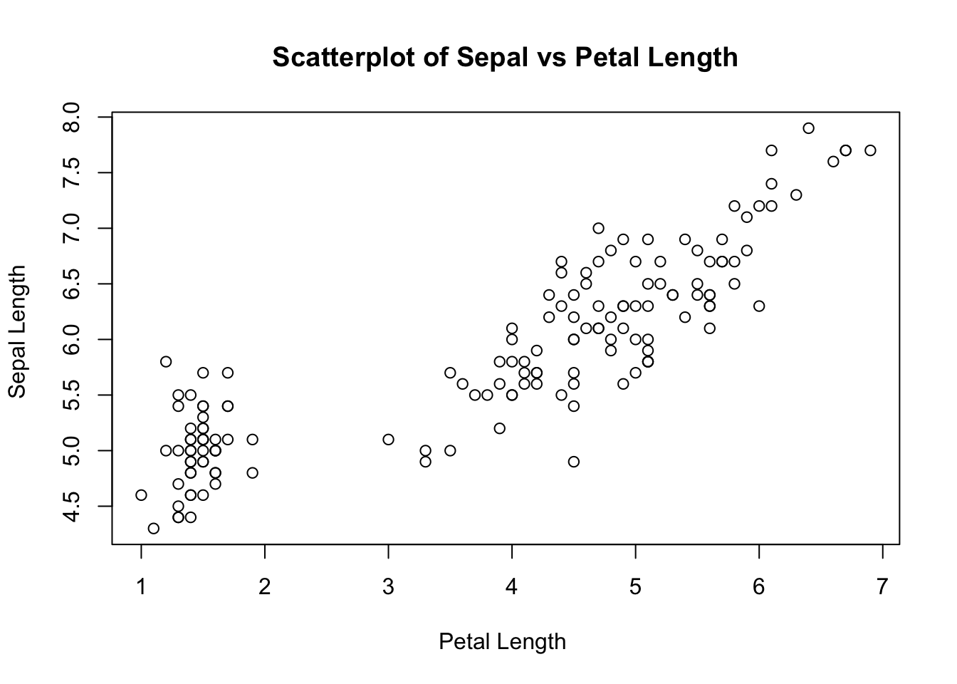
1.7 Making scatter matrix plots
Sometimes when we want to plot all or most of the numeric columns in the dataset at once. In this plot we removed the categorical variable Species. This can us quickly understand relationship between different features.
But we have to be careful when there are many variables. Because plotting many variables at once can make the plot look dirty and clumnsy. In this example we can see that Petal.Length and Petal.Width have a strong relationship.
1.8 Using GGplot2 to plot and explore dataset
ggplot2 is a R package that is very useful for plotting. Install the package by typing install.packages("ggplot2") and then load the library library(ggplot2). We only need to install a package in the computer once, but need to load the library everytime we run R. This package is much more extensive in plotting compared to the base plot in R and can produce beautiful plots. To learn more about ggplot2 visit https://ggplot2.tidyverse.org/ or learn from Hadley Wickham’s GGPlot book.
Lets explore some data using plot
library(ggplot2)

# scatterplot with colors
ggplot(iris, aes(x= Sepal.Length, y = Petal.Width, color = Species))+
geom_point() 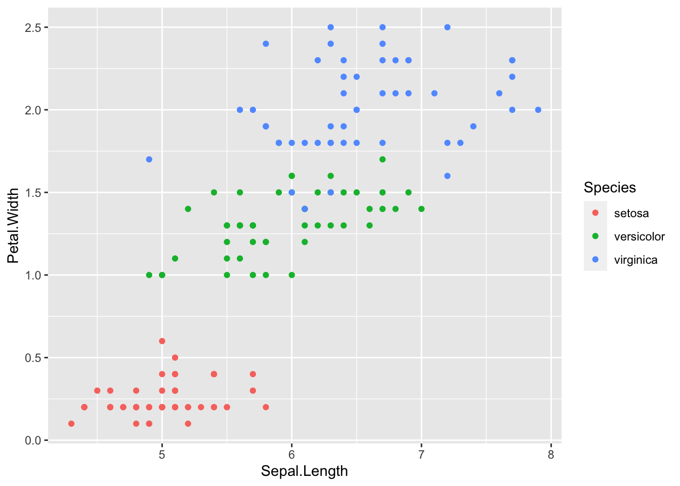
#Scatterplot to visualize 3 variables

ggplot(iris, aes(x = Sepal.Length, y = Petal.Length,color = Species))+
  geom_point() + geom_smooth(method = lm)+ geom_jitter()
## `geom_smooth()` using formula 'y ~ x'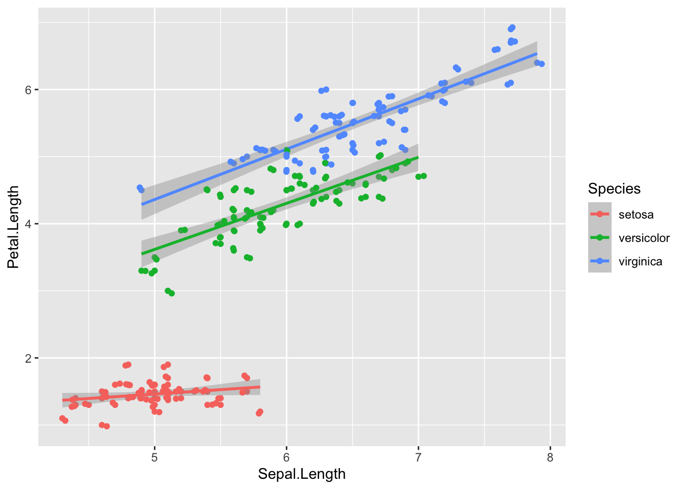
#frequency polygon
ggplot(iris, aes(x = Petal.Width, color = Species))+ geom_freqpoly(binwidth =0.1)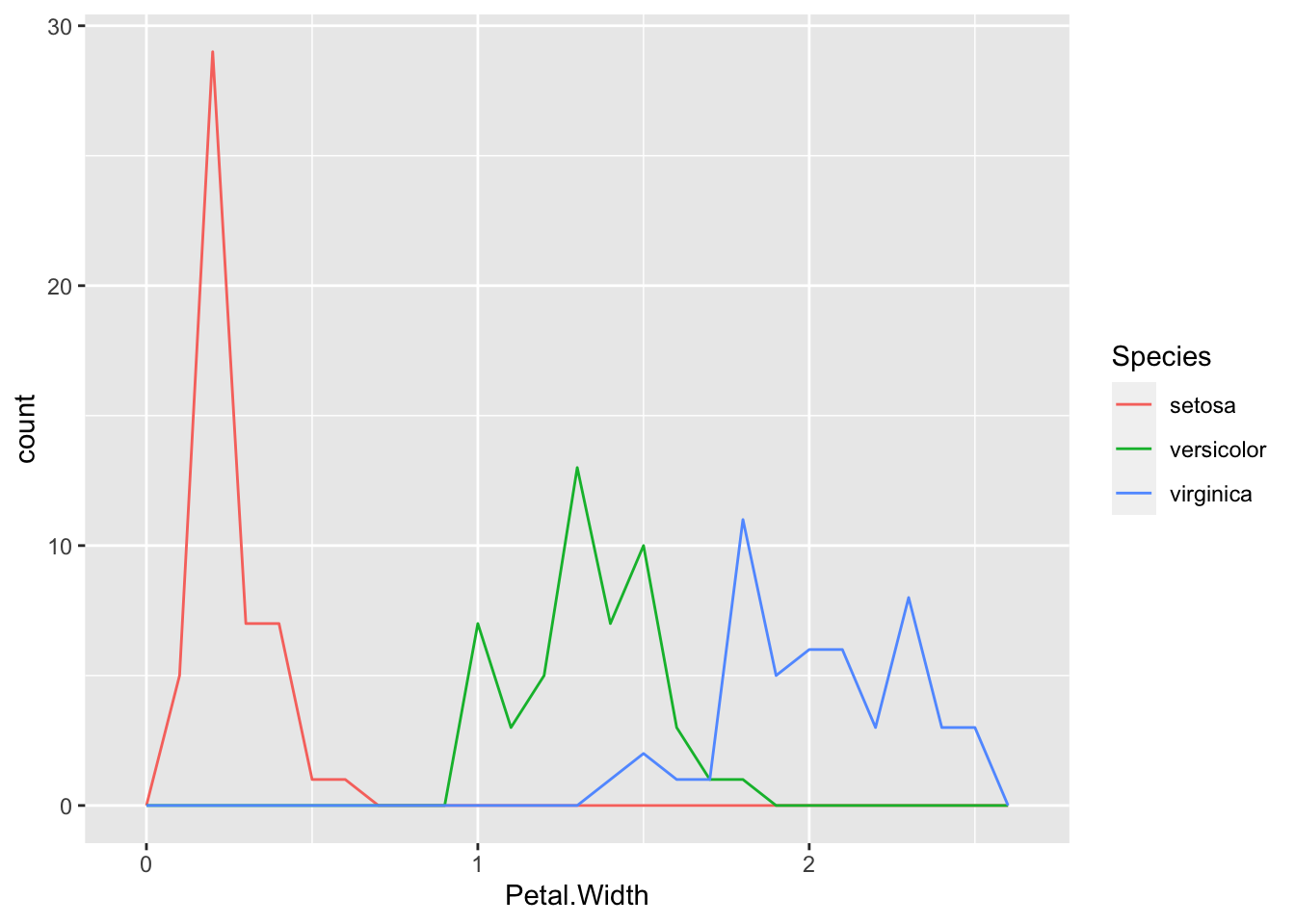
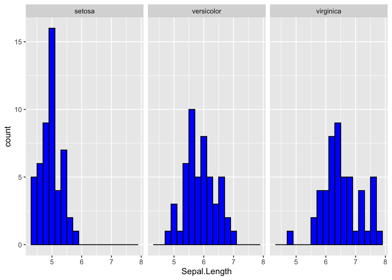
#Histogram of Sepal Length by Species. visualizing two variables in histogram using subplots
ggplot(iris, aes(x= Sepal.Length))+ geom_histogram(col= "black", fill = I("blue"), binwidth = .2)+
  facet_wrap(~Species)